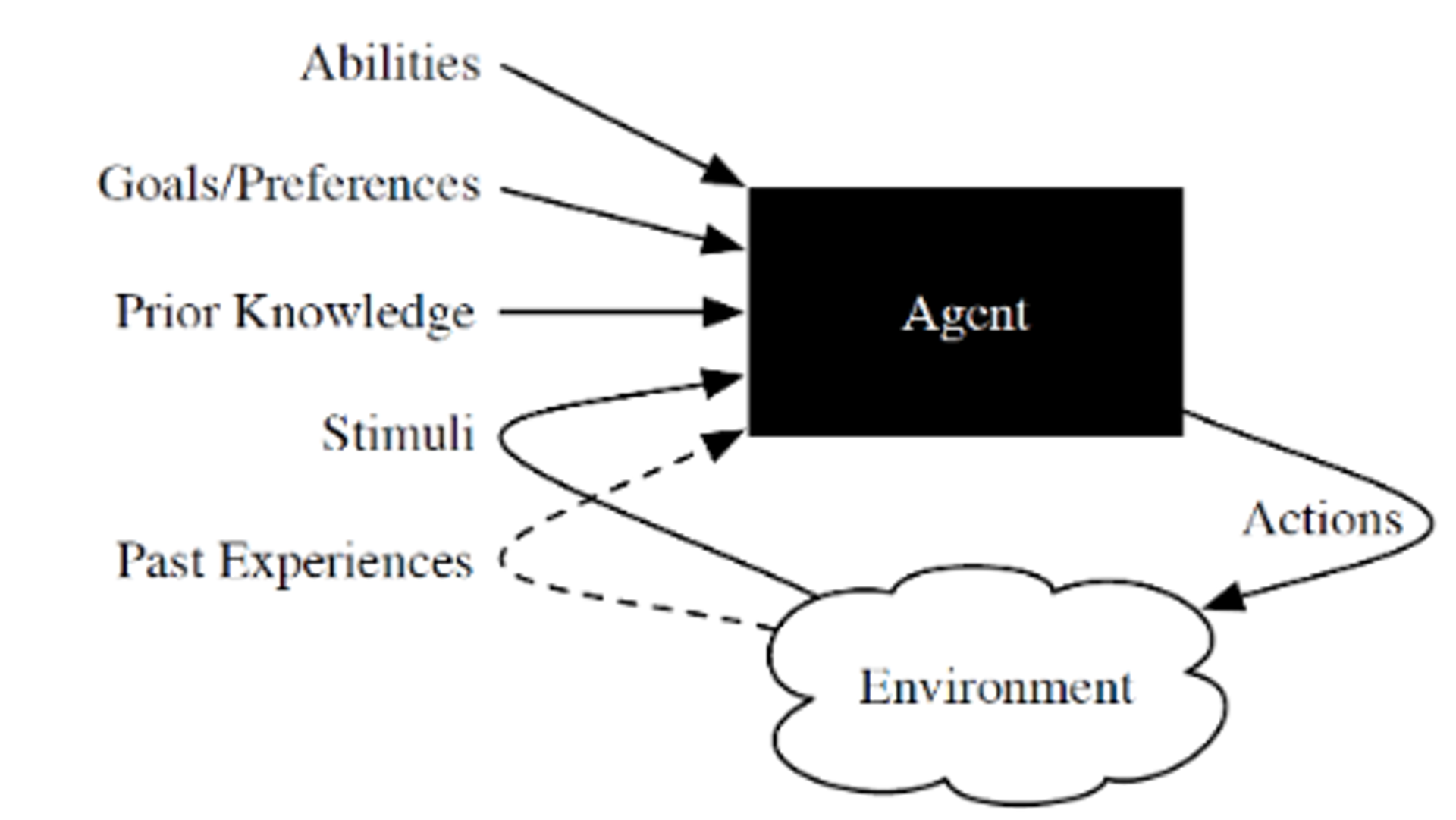

Our goal is to build a useful, intelligent agent
Are the state / action / percept spaces finite?
Are there other agents interacting?
Can the world change while the agent is "thinking"?
Note: The classification sometimes depends on time discretization. In this example, 1 time step = a single move by the agent & opponent.
Adversarial search problem or zero-sum game - covered in Module 5
🧠 Why is this? Because it's fully observable (Percept function is the identity function)
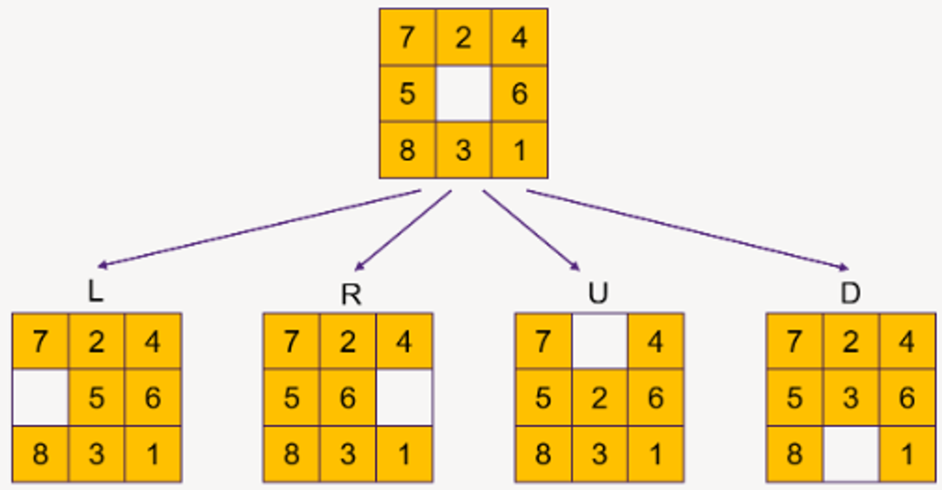
Goal: How to find the solution with the smallest exploration cost?
For this module of the course, we will discuss two types of search:
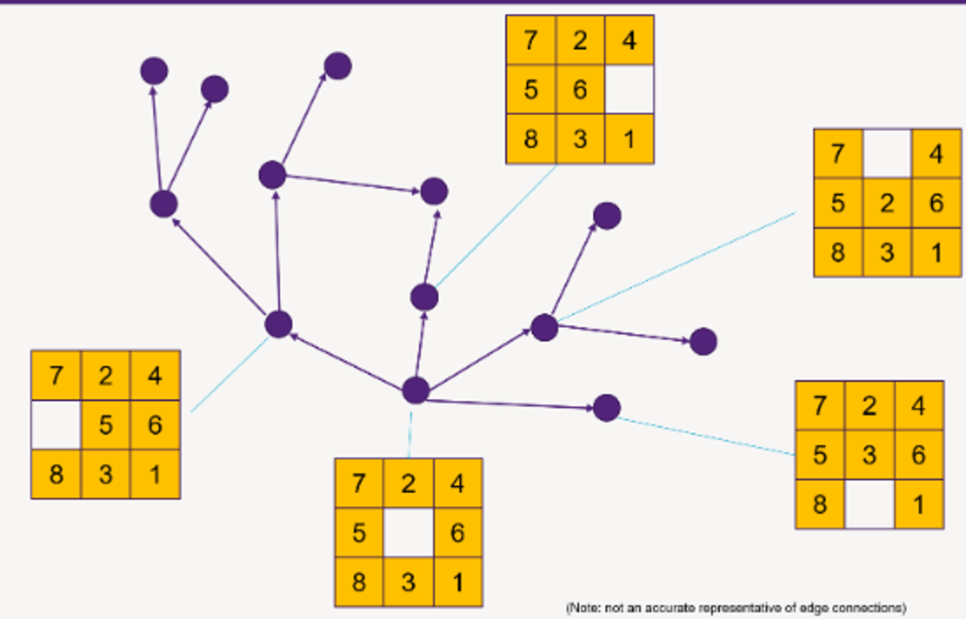
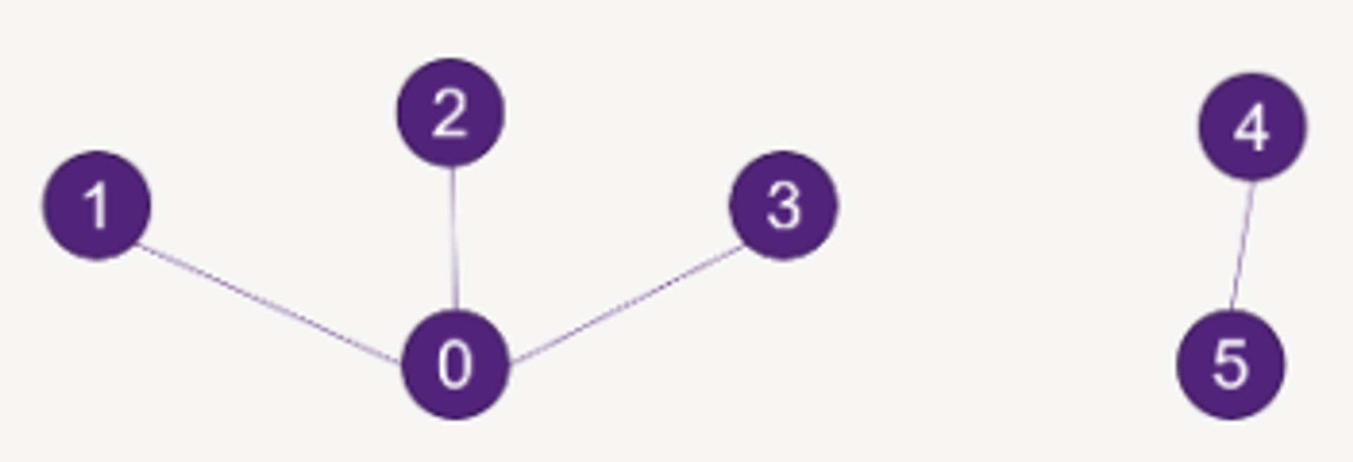
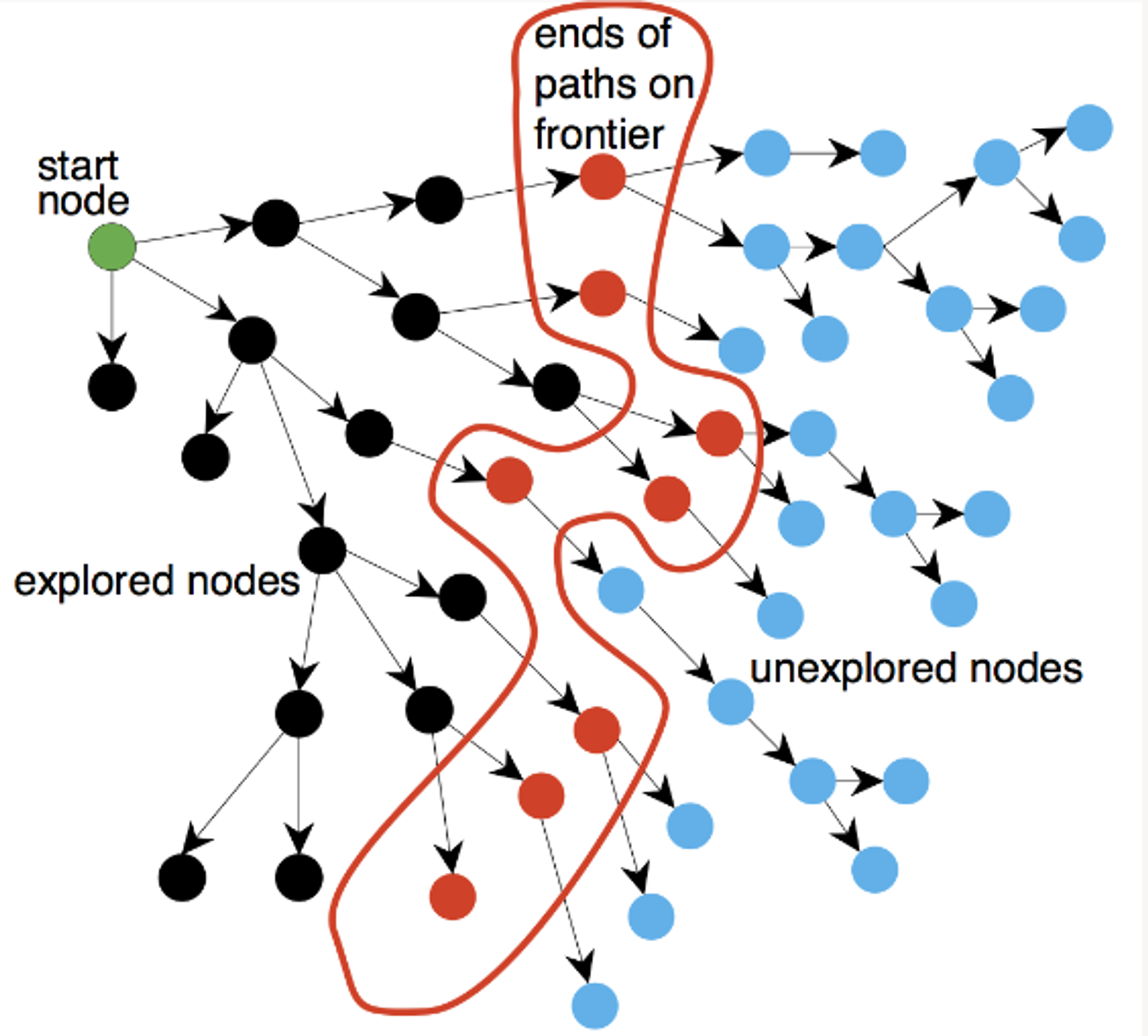
v from the containerv is the goal vertex, then returnv (i.e. put the results of successor(v) to the container)successor(v) is a function that:
v as inputv (i.e. the end-point of out-edges from v)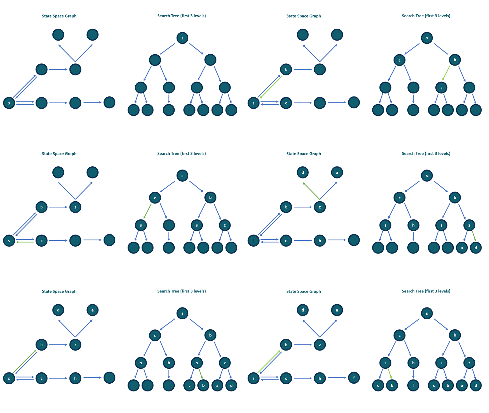
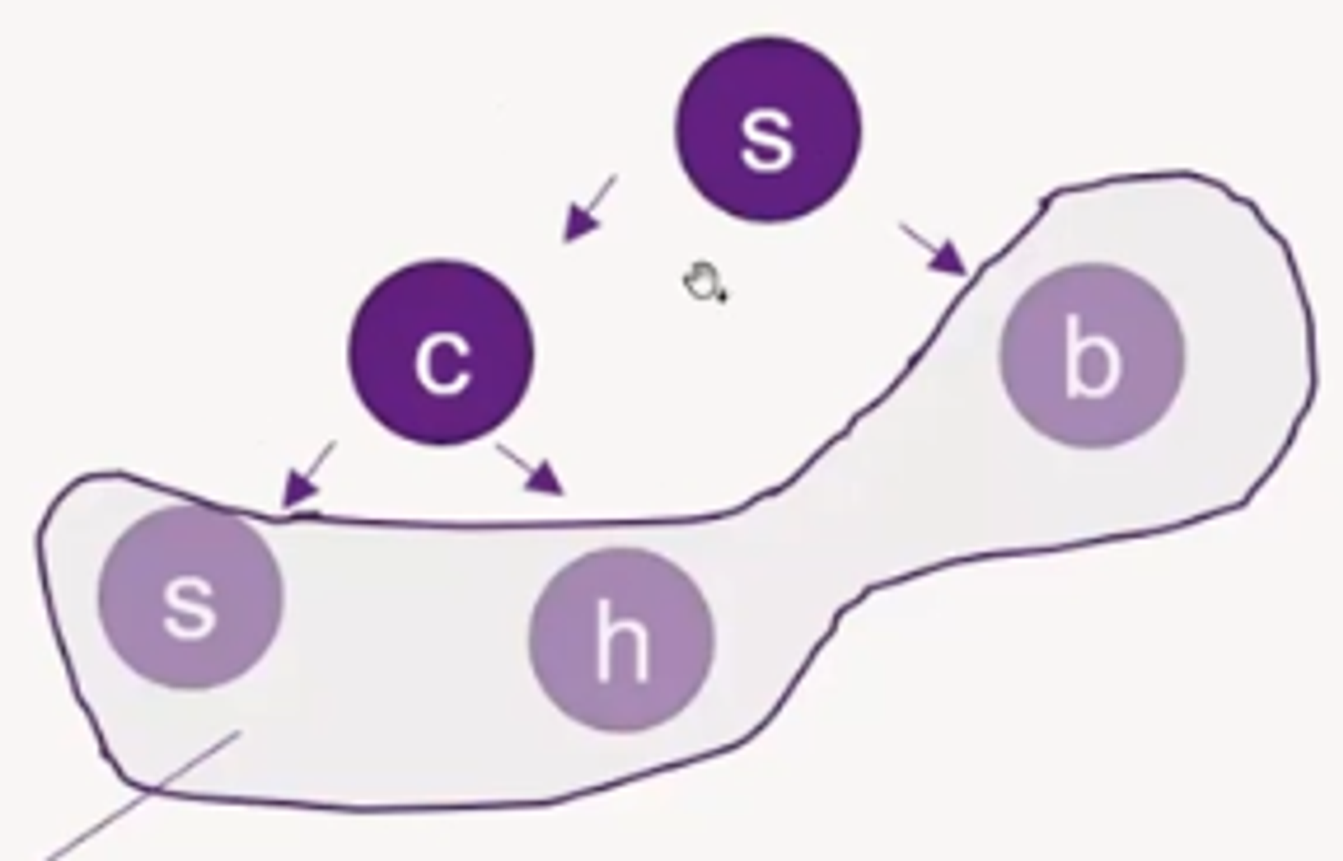
t from the fringe.t is the goal vertex, then return.t (i.e., put the results of successor(t) into the "container").successor(t) again. Now vertex v of the state graph corresponds to a node t in the search tree, so successor(t) are the children of t in the search tree.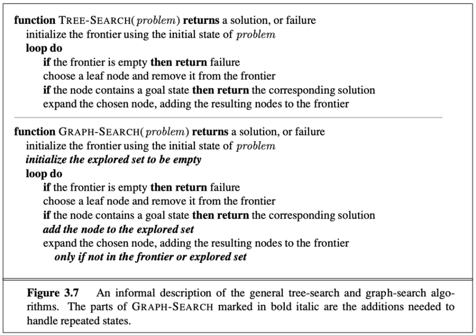
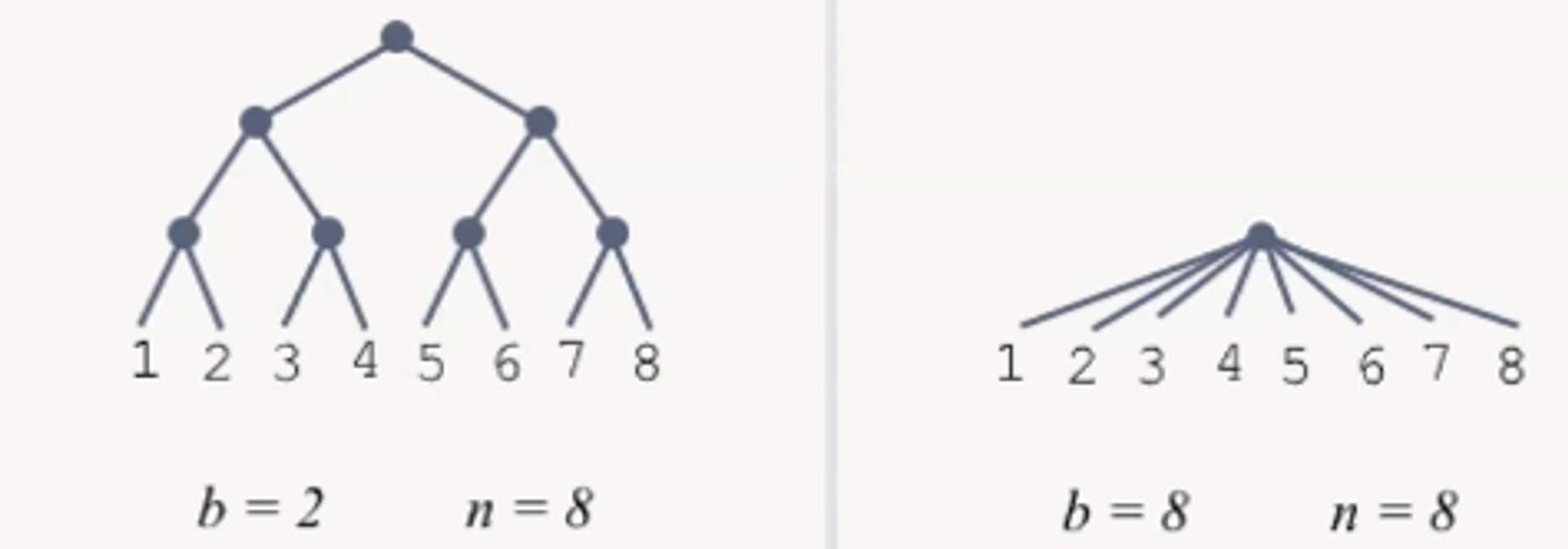
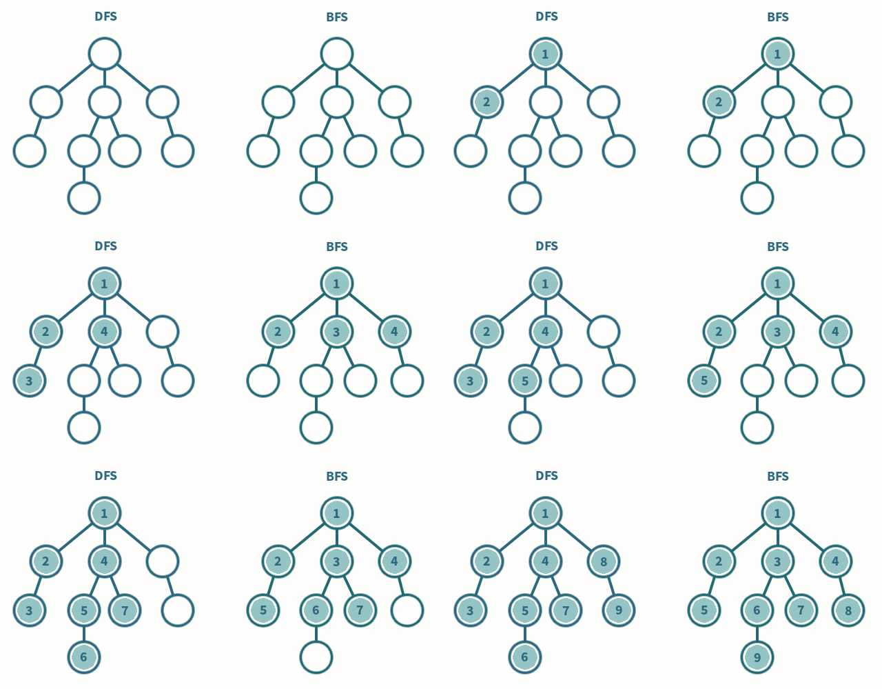
b branching factord depth of shallowest goal nodeComplete (Will BFS find a solution?)
Generate optimal solution (Does BFS guarantee to find the path with the fewest edges?)
Complexity: How does it scale in relation to the branching factor and the depth of the shallowest goal node
(Where
b branching factorm maximum depth of treed depth of shallowest goal nodeComplete (Will DFS find a solution?)
Generate optimal solution (Does DFS guarantee to find the path with the fewest edges?)
Complexity
BFS Finds minimum step path, but requires exponential space
DFS Efficient in space O(m) but no path length guarantee
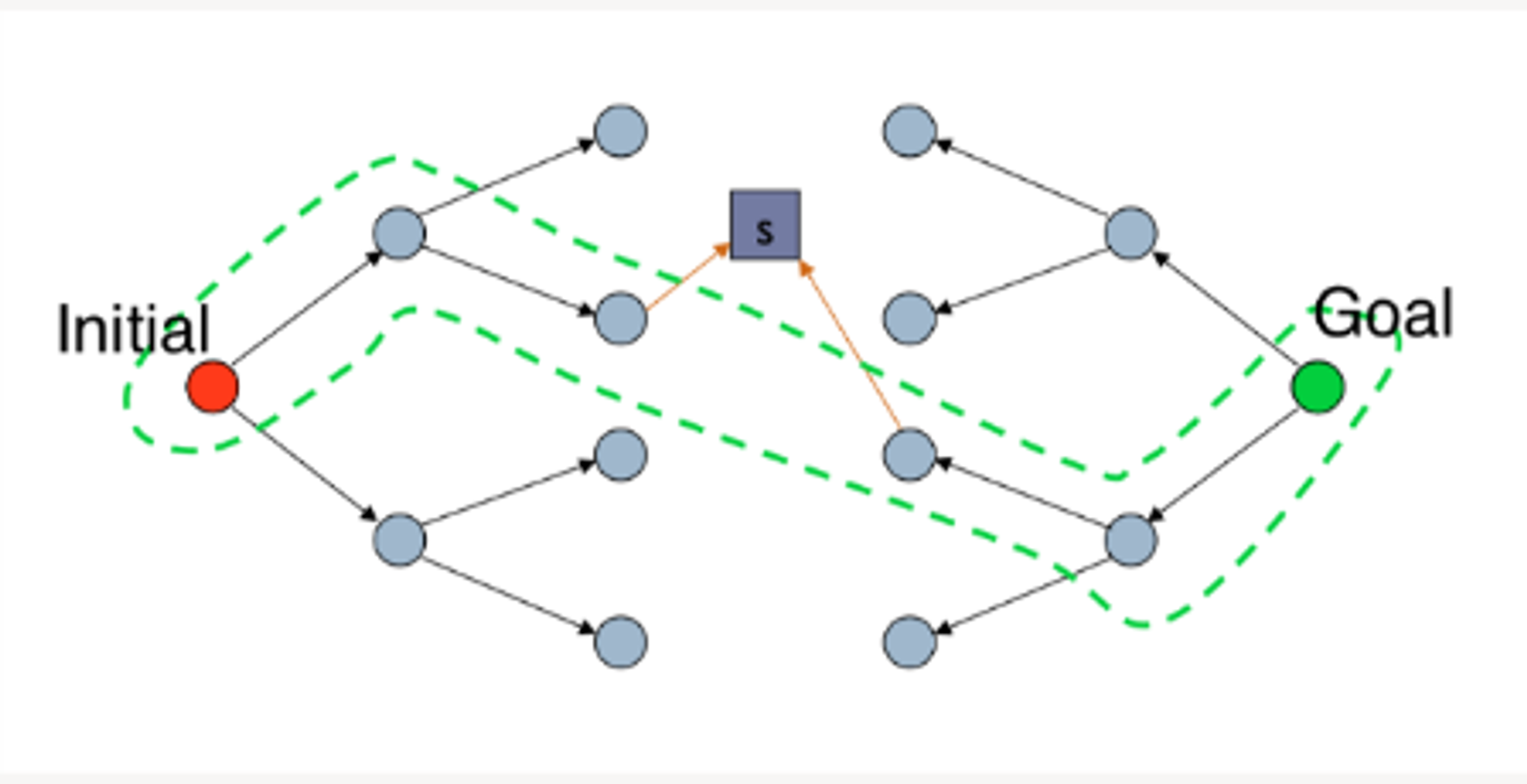
IDDFS Multiple DFS with increasing depth-cutoff until the goal is found
For
Only generates nodes with depth
Parameters:
Complete (will DFS find a solution?)
Generate optimal solution (Does IDDFS guarantee to find the path with the fewest edges?)
Complexity
Expanding geometric sequence
Breadth-First SearchUniform Cost Search treats the frontier as a priority queue, ordered by path cost.import queue
q = queue.PriorityQueue()
Complete Will UCS find a solution?
Generate optimal solution Does UCS guarantee to find the path with the lowest cost?
Complexity