Lecture 06

1.0 - Graph Data Structures

We may need certain information about graphs:

Shortest path from vertex $v$ to vertex $u$
Shortest path from vertex $v$ to every other vertex (typically require this to solve previous)
Does the graph contain cycles?
Is it connected?
Find a minimum spanning tree
Shortest tour of all vertices? (shortest path through all vertices)

Graphs will be used to explore different programming styles throughout the course.

1.1 - Types of Graphs

Directed Acyclic Graphs (DAGs)
Connected Graphs
Trees are special types of graphs
Lists and vectors are also simple graphs.

1.2 - Graph Representations

There are two main approaches to representing graphs:
- Adjacency Lists
- Adjacency Matrix
(Representing the set of vertices and edges directly is too inefficient)

1.2.1 - Adjacency List (Undirected)

🌱 For every vertex, store a list of vertices that it’s adjacent to

Node	Connections
A	B, C, D
B	A, D
C	A, D
D	A, B, C

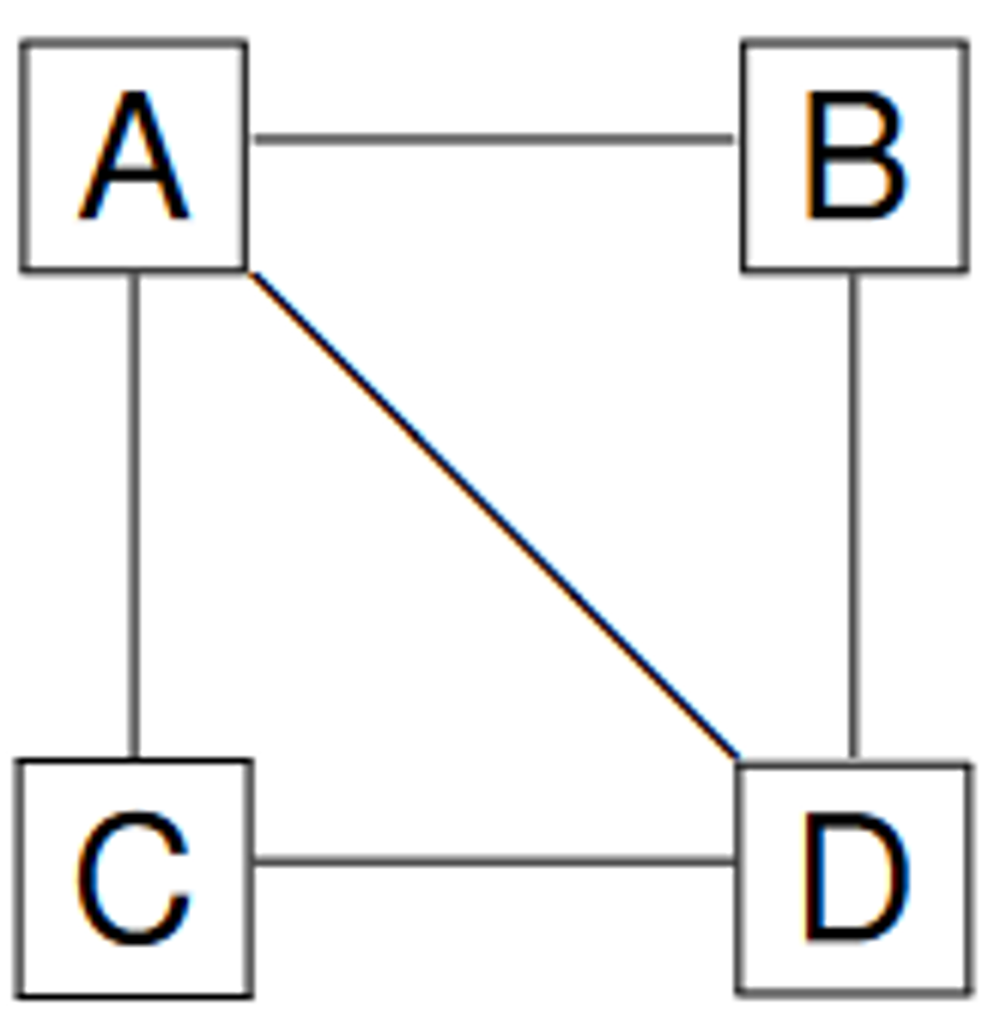
For an undirected graph $G=(V, E)$ with $\bold{V}$ vertices and $\bold{E}$ vertices, what is the worst-case:

Space Complexity is proportional to the number of vertices and edges - For every vertex, we store a list of the adjacent vertices of size $\text{degree(v)}$ . $\sum_{v\in G.V} \text{degree(v)}=2E$ as in an undirected graph, we count every edge twice (as $a$ is in $b$ ’s adjacency list and vice versa).

$\Theta(V+\sum_{v\in G.V} (\text{degree(v)})=\Theta(V+2E)=\Theta(V+E)$
Time Complexity of isAdjacentTo(u, v) We find the adjacency list for $u$ ( $\Theta(1)$ ), and iterate through it to find $v$ (worst case $\Theta(V)$ )

$\Theta(V)$
Time Complexity to list all adjacent vertex pairs Have to iterate through every entry in each adjacency list - in worse case $V^2$ time in the case of a dense graph (with many edges). However, we know that all of the adjacency lists contain a maximum of $\Theta(2E)$ entries.

$\Theta(V+\sum_{v\in G.V}\text{degree(v)}=\Theta(V+2E)=\Theta(V+E)$

1.2.2 - Adjacency List (Directed)

Node	Connections
A	B, D
B	D
C	A
D	C

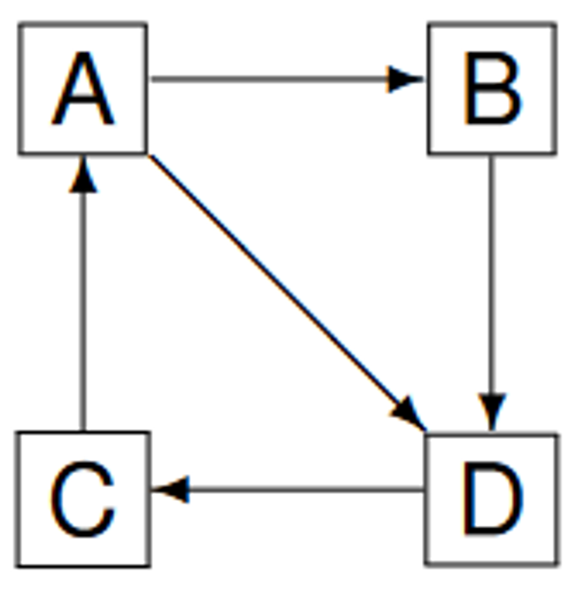
For a directed graph $G=(V,E)$ with $\bold{V}$ vertices and $\bold{E}$ vertices, what is the worst-case:

Space Complexity is proportional to the number of vertices and edges - Each adjacency list contains all of the destinations of each edge.

$\Theta(V+\sum_{v\in G.V} \text{outDegree(v)})=\Theta(V+E)$
Time Complexity of isAdjacentTo - same analysis as for an undirected graph - $\Theta(1)$ lookup of adjacency list, and $\Theta(V)$ worst case lookup

$\Theta(V)$
Time Complexity to list all adjacent vertices

$\Theta(V+\sum_{v\in G.V} \text{outDegree(v)})=\Theta(V+E)$

1.2.3 - Adjacency Matrix (Undirected)

	A	B	C	D
A	❌	✅	✅	✅
B	✅	❌	❌	✅
C	✅	❌	❌	✅
D	✅	✅	✅	❌

For an undirected graph $G=(V, E)$ with $\bold{V}$ vertices and $\bold{E}$ edges what is the worst case:

Space Complexity as we have to create a $V\times V$ matrix

$\Theta(V^2)$
Time Complexity of isAdjacentTo(u, v) as we just index into the matrix for both entries

$\Theta(1)$
Time Complexity to list all adjacent vertex pairs as we have to iterate through every cell of the matrix.

$\Theta(V^2)$
Observe that the adjacency matrix of an undirected graph is symmetric about the diagonal

1.2.4 - Adjacency Matrix (Directed)

	A	B	C	D
A	❌	✅	❌	✅
B	❌	❌	❌	✅
C	✅	❌	❌	❌
D	❌	❌	✅	❌

For a directed graph $G=(V, E)$ with $V$ vertices and $E$ edges, what is the worst-case

Space Complexity as we have to create a $V\times V$ matrix

$\Theta(V^2)$
Time Complexity of isAdjacentTo(u, v) as we just index into the matrix for both entries

$\Theta(1)$
Time Complexity to list all adjacent vertex pairs as we have to iterate through every cell of the matrix.

$\Theta(V^2)$

1.3 - Comparison of Graph Representations

The adjacency list representation is often the most efficient if the graph is sparse:
- Few edges relative to the number of vertices
The adjacency matrix representation is often the most efficient if the graph is dense:
- Many edges relative to the number of vertices.

2.0 - Graph Traversal Algorithms

2.1 - Graphs and Shortest Path Algorithms

For an unweighted graph $G$ $G$
- The length of a path is the number of edges in that path.
- For example, the length of $\langle v_1, v_2, v_3\rangle$ is 2
The distance from vertex $v$ to $u$ is the length of the shortest path from $u$ to $v$ in $G$ .

2.2 - Breadth-First Search

Takes as an input an unweighted graph $G=(V, E)$ and a designated start vertex $v\in G.V$
Traverses vertices in $G$ in order of their distance from $v$
Finds the shortest paths from $v$ to every other vertex in $G$

2.2.1 - Implementation of BFS

What do we know about BFS?

Start vertex $v$ is at a distance $0$ from itself.
The vertices adjacent to $v$ , other than those at distance $0$ are at distance 1
The vertices adjacent to v’s adjacent vertices (other than those at distance 0 or 1
etc…

We will use a queue data structure:

Vertices are:
- Enqueued in order of their distance from the start vertex
- Dequeued in order of their distance from the start vertex
The first element added to the queue is the start vertex
When a vertex is dequeued, its adjacent vertices that have not yet been reached are enqueued
Can be implemented either using a circular array (require amortisation to resize), or a linked list

How do we keep track of which vertices have been reached?

Colours are used to distinguish vertices at different stages within an algorithm:
- White Not yet reached (never enqueued, a shortest path not yet found)
- Grey Reached, but all adjacent vertices not reached yet (i.e. enqueued, but not dequeued; a shortest path found)
- Black Reached and completed (i.e. enqueued and dequeued; shortest path found)

🌱 To find the shortest path from A to B, we just need to keep track (update) of the parent of each node as we visit it

BFS(G, v)
for u in G.V - {v} # For all but the starting vertex.
		u.distance = ∞;
		u.colour = white;
		u.parent = NULL;

v.distance = 0;
v.color = grey;
v.parent = NULL

Q.initialise()
Q.enqueue(v)

while !Q.isEmpty()
		current = Q.dequeue()
		for u in G.adjacent[current]
				if u.colour == white # For vertices with no shortest path yet, compute.
						u.distance == current.distance + 1
						u.color = grey;
						u.parent = current
						Q.enqueue(u)
		current.color := black

2.2.2 - Performance of BFS

The worst-case time complexity of BFS is:

$\Theta(V)+\Theta(1)+(\sum_{v\in G.V} \Theta(1)) + \text{outDegree}(v)\times\Theta(1))=\Theta(V+E)$

The worst-case space complexity of BFS is $\Theta(V)=\Theta(V)+\Theta(V)$ (for space to store colours, and the queue).

Assuming enqueue and dequeue take $\Theta(1)$ time, and we use an adjacency list representation of our graph problem - require determining adjacent vertices in $\Theta(\text{outDegree(v)})$ time.

That is:

$\Theta(V)$ for initial colouring

$\Theta(1)$ for setup of initial vertex v, initialisation of queue and enqueueing v.

$\sum_{v\in G.V}\Theta(1)+\text{outDegree(v)}\times\Theta(1)$ as:

Each vertex can be added to the queue at most one time; Therefore, the while loop iterates at most $\Theta(V)$ times.

We perform the inner loop $\text{outDegree(v)}$ times, in which we do a constant amount of work per iteration of the inner loop.

Since $\sum(\text{outDegree(v)})=\Theta(E)$

2.3 - Depth-First Search

Doesn’t necessarily find the shortest paths
Often used as a sub-routine within other algorithms
Typically use DFS to learn more about the structure of a graph
A recursive algorithm that visits a vertex $v$ $v$ by:
- Choosing an unvisited vertex adjacent to v
- visiting $u$ and so on
- Before backtracking to $v$ , and continuing until $v$ has no more unvisited adjacent vertices.

2.3.1 - Implementation of DFS

We store additional information about the graph by storing a node’s parent so that we can re-create the traversal path taken
A depth-first search on an undirected graph produces a classification of the edges of the graph into tree edges, or back-edges
- For a directed graph, there are further possibilities.

The depth-first search algorithm can be used to classify the edges in a graph (directed) into four types: (in an undirected graph, we only have tree edges and back edges)

Tree Edges If the procedure DFS(u) calls DFS(v) then (u, v) is a tree edge.
Back Edges If the procedure DFS(u) explores the edge (u, v), but finds that v is an already-visited ancestor of u, then (u, v) is a back edge.
- If a graph has a back edge, then it is cyclic.

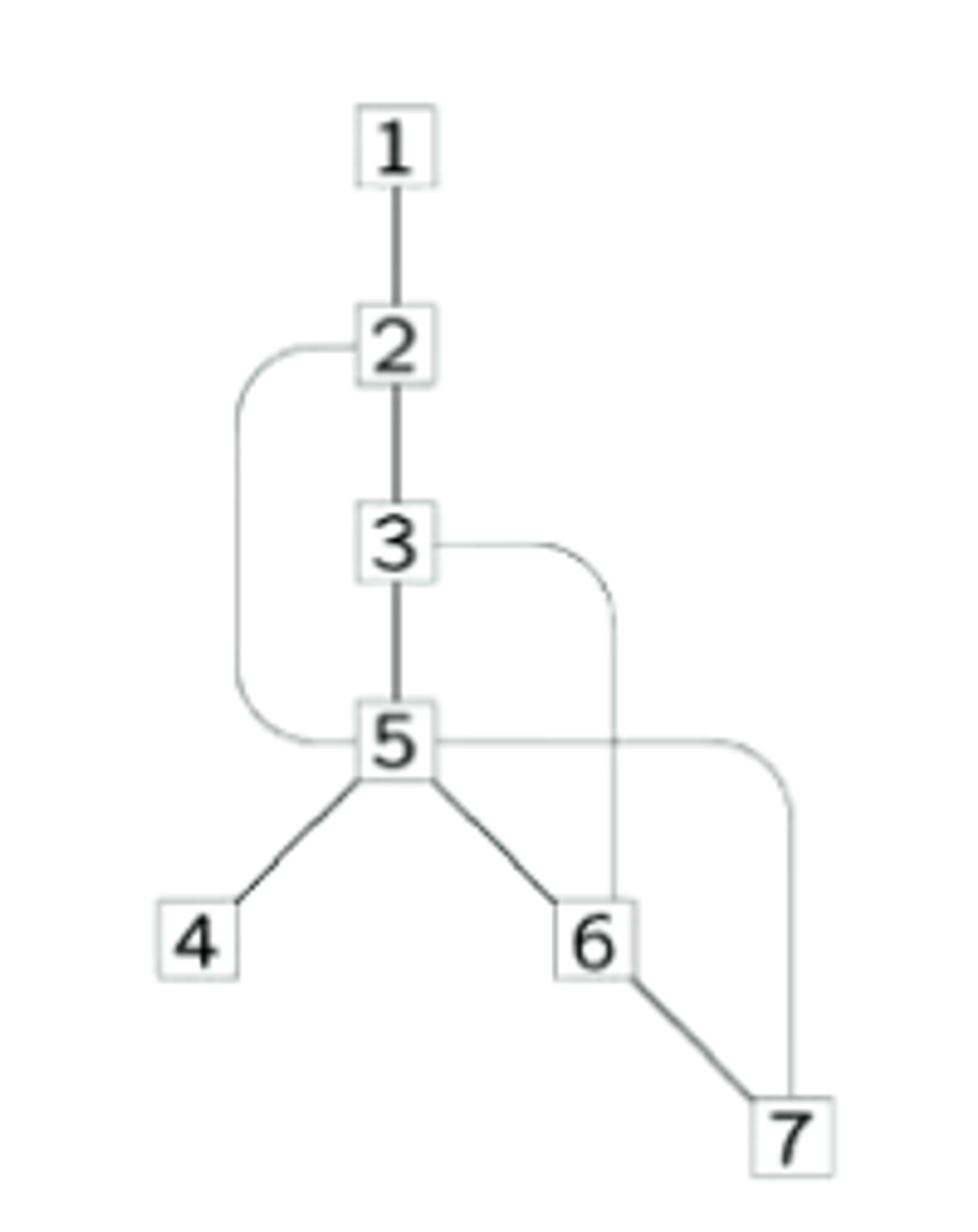
DFS Graph with back-edges (thinner lines)

Forward Edges If the procedure DFS(u) explores the edge (u, v) but finds that v is an already visited descendant of u, then (u, v) is a forward edge
Cross Edges All other edges are cross-edges.

DFS(G):
	# We use colour to indicate where in the traversal process we are
	for u in G.V 
			u.color = white
			u.parent = NULL
  # For each vertex, we call dfs_visit on it
	for u in G.V
		if u.color == white then DFS_Visit(G, u)

DFS_Visit(G, v)
	v.color = grey # Started traversal, but not finished
	for u in adjacent[v]
		if u.color == white:
				u.parent = v
				DFS_Visit(G, u)
	v.color = black # Finished traversal for v

2.3.2 - Performance of DFS

$\Theta(V)$ for initial colouring

$\Theta(V)+\color{pink}x$ Each vertex can only be visited once, as we only visit it when it is coloured white.

$\color{pink}\sum_{v\in G.V}$ work for the for loop in DFS(G), calling DFS_Visit for each vertex.

$\color{pink} \Theta(1)$ work for setting colours to grey and black at the start and end of the method

$\color{pink}\text{outDegree(v)}$ work for the for loop - a vertex has $\text{outDegree(v)}=\Theta(E)$ adjacent vertices.

Therefore, the work done (time complexity) by DFS is given as:

$\Theta(V)+(\sum_{v\in G.V}\Theta(1)+\text{outDegree(v)}\times\Theta(1))=\Theta(V+E)$

We use $\Theta(V)$ space to store the colours of each node, and $\Theta(V)$ space for recursive calls

$\Theta(V)$ space for stack frame of recursive calls. In the worst case, the depth of the graph is $V$ .

2.3.3 - DFS with Start and Finish Times

DFS(G):
	time = 0
	# We use colour to indicate where in the traversal process we are
	for u in G.V 
			u.color = white
			u.parent = NULL
  # For each vertex, we call dfs_visit on it
	for u in G.V
		if u.color == white then DFS_Visit(G, u)

DFS_Visit(G, v)
	time += 1
	u.discovered = time
	v.color = grey # Started traversal, but not finished
	for u in adjacent[v]
		if u.color == white:
				u.parent = v
				DFS_Visit(G, u)
	v.color = black # Finished traversal for v
	time += 1
	u.finished = time

3.0 - Directed Acyclic Graphs

A directed acyclic graph (DAG) is a directed graph with no cycles
The vertices in a DAG can be thought of as tasks
The directed edges in a DAG can be thought of as dependencies between vertices (tasks)
A topological sort of a directed acyclic graph $G=(V, E)$ is a linear ordering of $V$ , such that:
- if $(u, v)\in E$ , then $u$ comes before $v$ in the topological ordering
Given a directed acyclic graph, as shown below, we can generate a topological ordering of the graph.

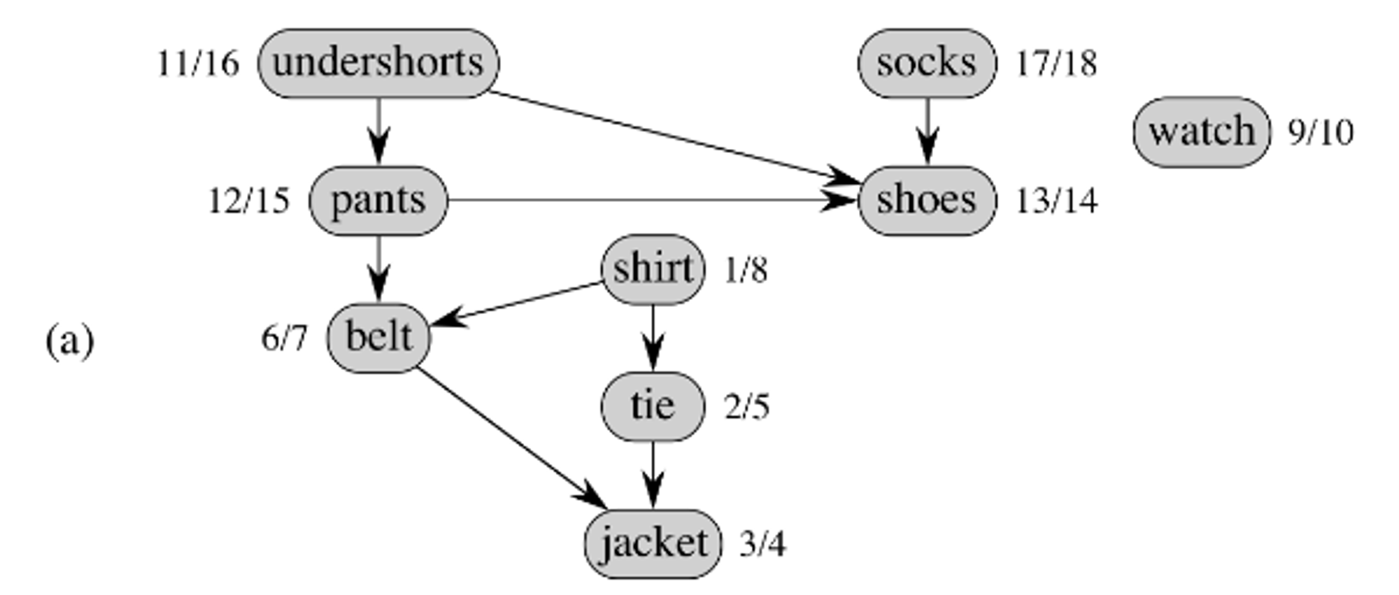
The following is a topological ordering of the above image

3.1 - Topological Sort

Performing a depth-first search on the graph will give a topological ordering.
- The starting and finishing times are listed on the side of each node {startTime}/{finishTime}

Topological_Sort(G):
    initialise an empty linked-list of vertices
		call DFS(G)
    as each vertex is finished in DFS, insert it onto the front of the linked list
    return the list of vertices.