1.0 - Minimum Spanning Trees
-
Consider laying cable (e.g. for the NBN)
- Create a connected network of houses that uses the least amount of cable.
- Assume that the speed of the cable is fast, i.e. the distance from house-to-house is irrelevant (we aren’t looking for the shortest paths
-
We are given an undirected, weighted graph with weights such that:
- Vertices represent houses to be connected to the NBN network
- For each edge , the weight is the cost of laying the cable from house to .
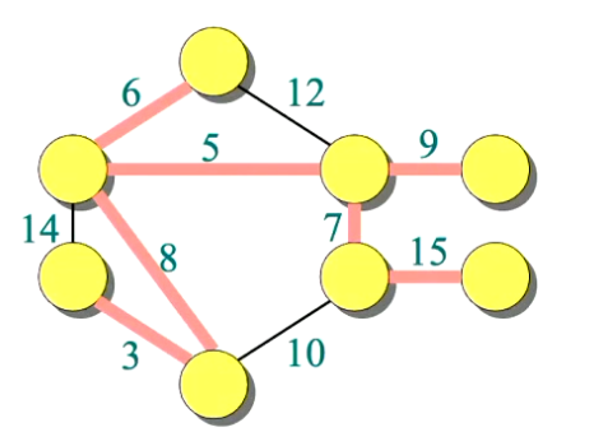
- We want to find an acyclic subset that:
- Connects all of the vertices in such that the total weight is minimised.
Inputs
- a connected, undirected, weighted graph
- Weights , where is the weight of the edge from to
Output
-
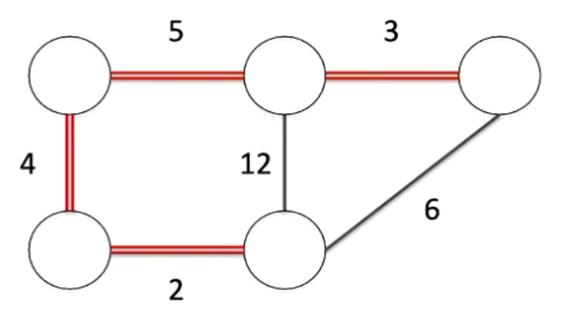
a subset of , that forms a spanning tree (connected acyclic subgraph of ) that contains all vertices of (spanning) and is of minimal weight:
-
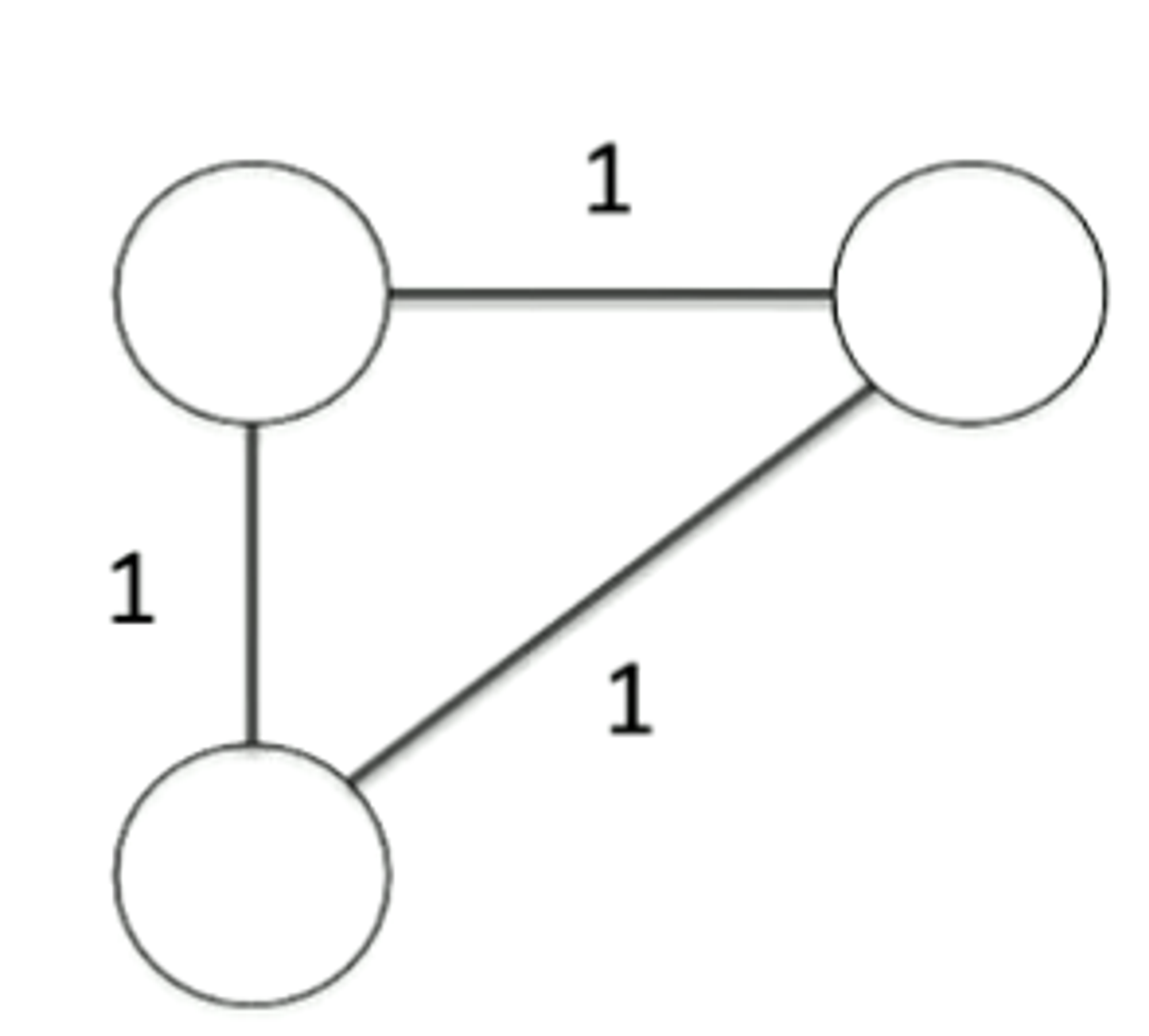
The smallest connected, undirected, weighted graph with more than one minimum spanning tree are three connected vertices, with equally weighted edges.
1.1 - Generic Construction of a MST
💡 Incrementally construct T which is a set of edges, and which will eventually become a MST of G
genericMST(G, w):
  T = Graph() # Empty
  while T is not a spanning tree
		// invariant: T is a subset of some MST of G
    find an edge (u, v) that is safe for T // new edge added forms a new T that
                                           // is also a subset of a MST for the graph
    T = T ∪ {(u, v)}
  return T
- We want to figure out how to “greedily” choose edges to add to T - choose the edges in an efficient way.
1.1 - Prim’s Algorithm
🌱 Guaranteed to form a MST at the end of the algorithm if we choose least-weighted edges connected to our graph.
T is always a tree (a connected acyclic sub-graph of G):
-
Initially, T is chosen to contain any one vertex from G.V
-
At each step, the least-weight edge leaving T is added
-
The algorithm stops when T is spanning.
-
How do we (efficiently) find the least-weight edge leaving T?
-
Maintain a priority queue, Q containing vertices (all vertices that are not in tree)
-
For each :
- the least weight of an edge connecting v to T
- the vertex adjacent to v on that least-weight edge (parent)
-
Represent
where is the first vertex chosen for
1.1.1 - Priority Queues
A priority queue Q maintains a set S of elements, each associated with a key, denoting its priority
- In a min-priority queue, an element with the smallest key has the highest priority
Operations are available to:
insert(Q, x)Insert an element , with key into Qextract_min(Q)Removes and returns the element of Q with the smallest keydecrease_key(Q,x,k)decreases the key of x in Q to the value k
We have the possible implementations of priority queues, and their associated time complexities:
Unsorted List PQ
- Insert
- extract_min(Q)
- decrease_min(Q, x, k) given you have a reference to the object
Sorted List PQ
- Insert
- extract_min(Q) Remove element at start of list
- decrease_key(Q, x, k) Decrease key, re-sort list.
Heap (Complete Tree)
- Insert
- extract_min(Q)
- decrease_key(Q, x, k)
As it is a complete tree, the height of the tree
1.1.2 - Implementation of Prim’s Algorithm Using PQ
- Operates on a graph G, with weights w at a start vertex r
MST_Prim(G, w, r)
	for each v ∈ G.V
			// v.key: least edge weight connecting v to T
			v.key = infinity
			//vertex adjacent to v in T on least edge
      v.pi = NULL
	r.key = 0 // Initially set to highest priority in PQ
  while Q ≠ ∅
			// invariant: T is a subset of some MST of G
			//                where T = {(v, v.pi) : v \in V-{r}-Q
      u = extract_min(Q)
			// Need to re-compute the priority of edges in sub-MST
			// as we have changed the minimum spanning tree -priorities
			// might have changed
      for each v ∈ G.Adj[i] // "Edge relaxation process"
          if v ∈ Q and w(u, v) < v.key
							v.key = w(u, v) // Decrease the key
              v.pi = u
1.1.3 - Prim’s Algorithm in Practice
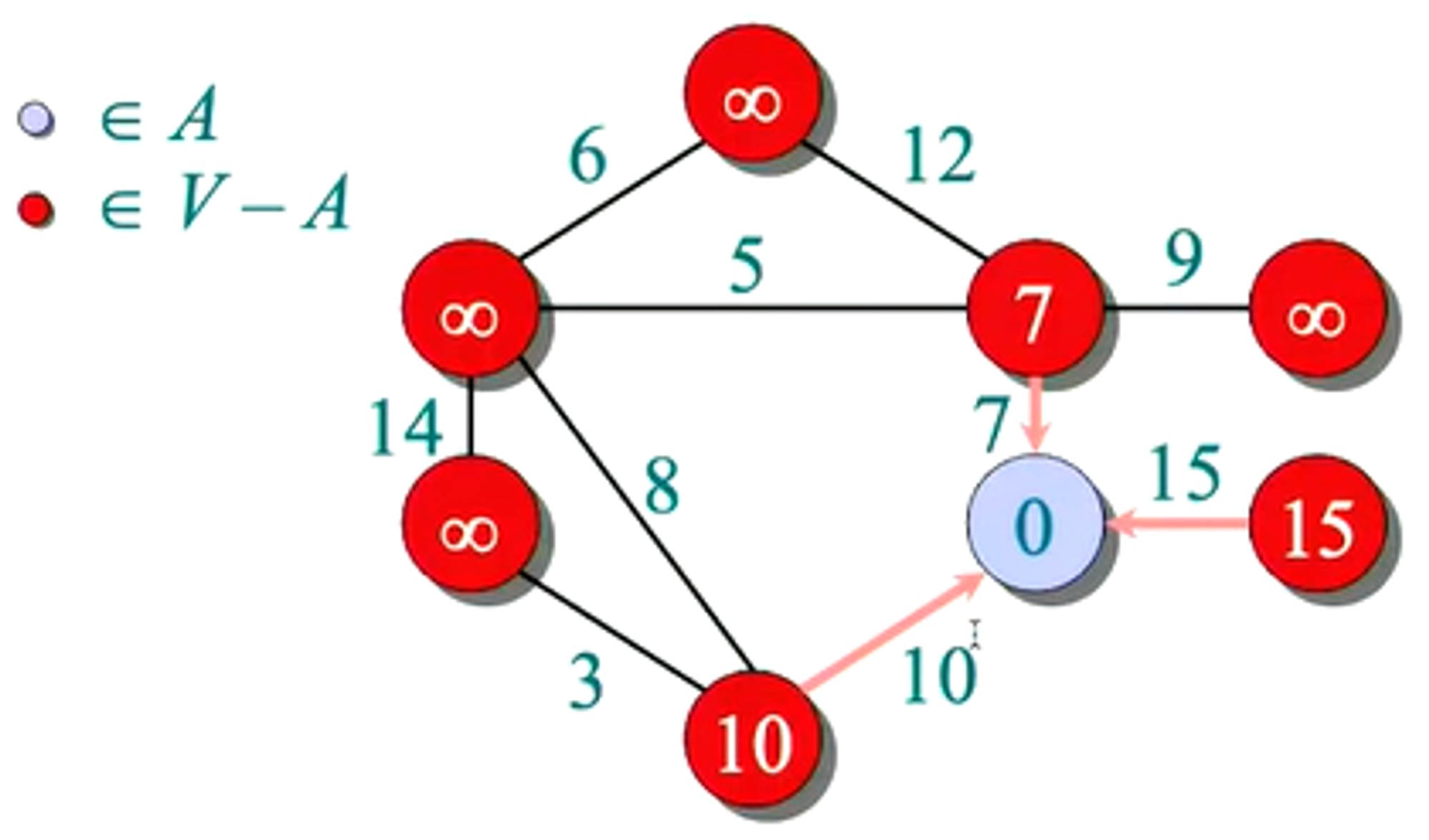
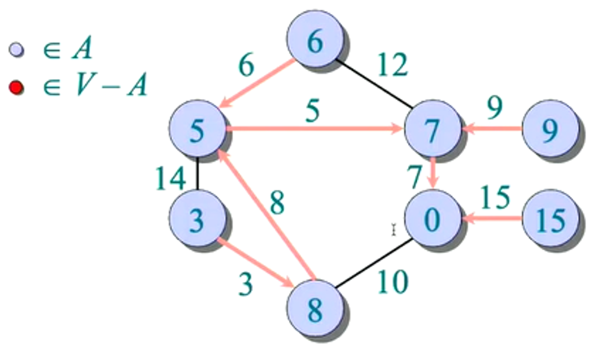
- Firstly begin with all vertices red (in the priority queue) with infinite weights, except for our initial vertex, which we assign a priority of 0.
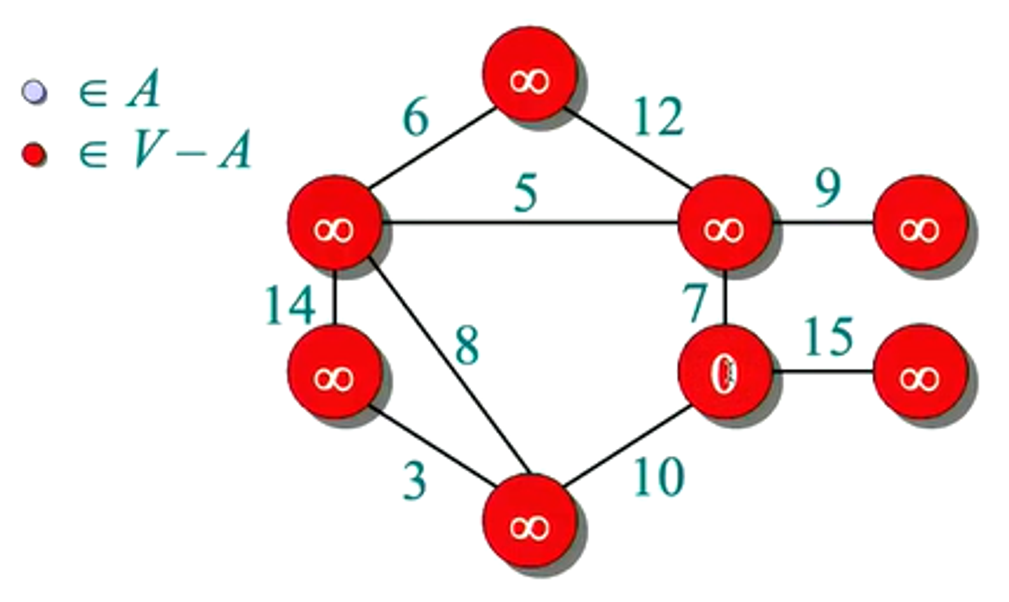
- We first remove the vertex with the highest priority
- Also, need to update the priority of the adjacent vertices using edge relaxation; improving weights
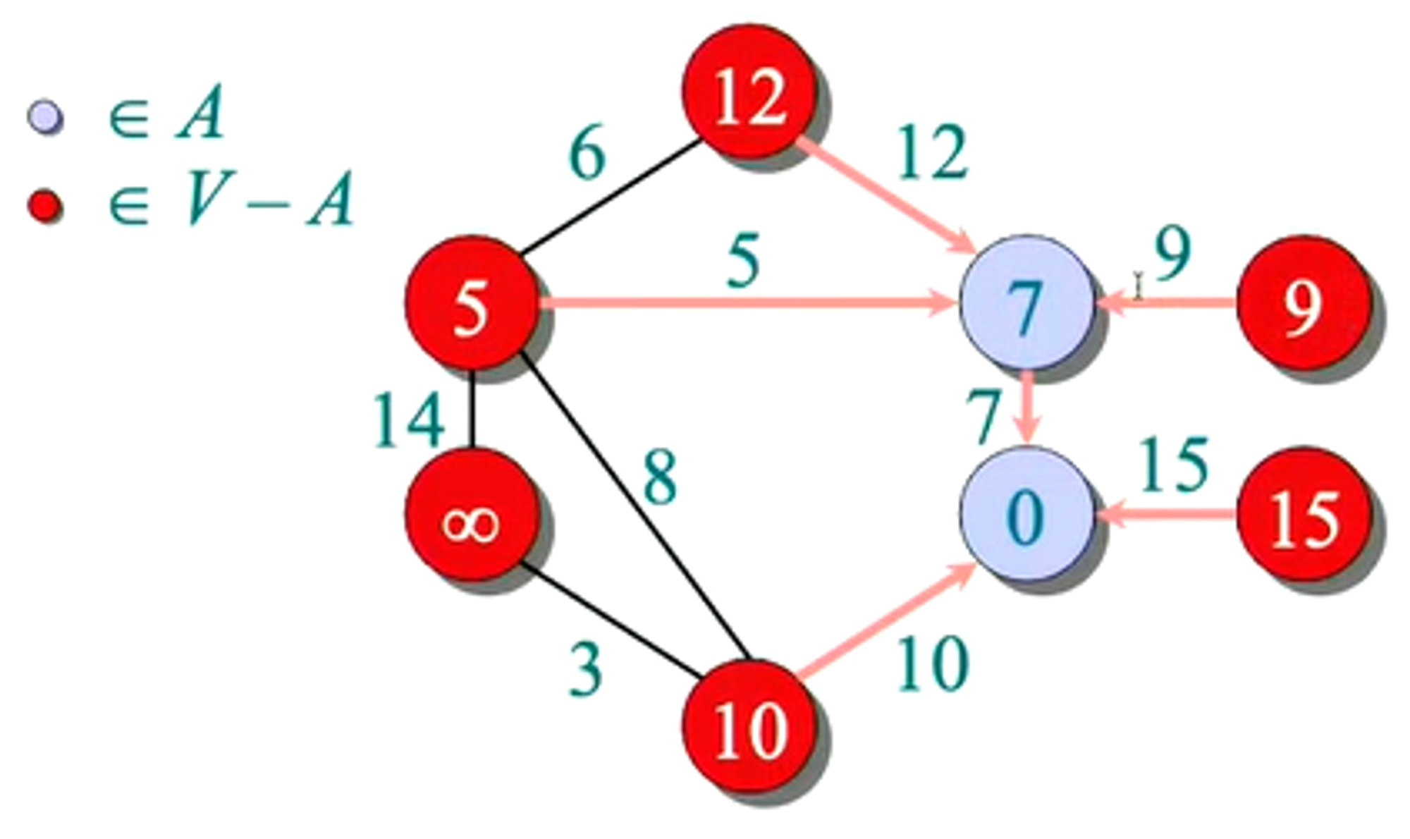
- Choose the next vertex with highest priority
- Update the weights of the vertices using the edge relaxation process
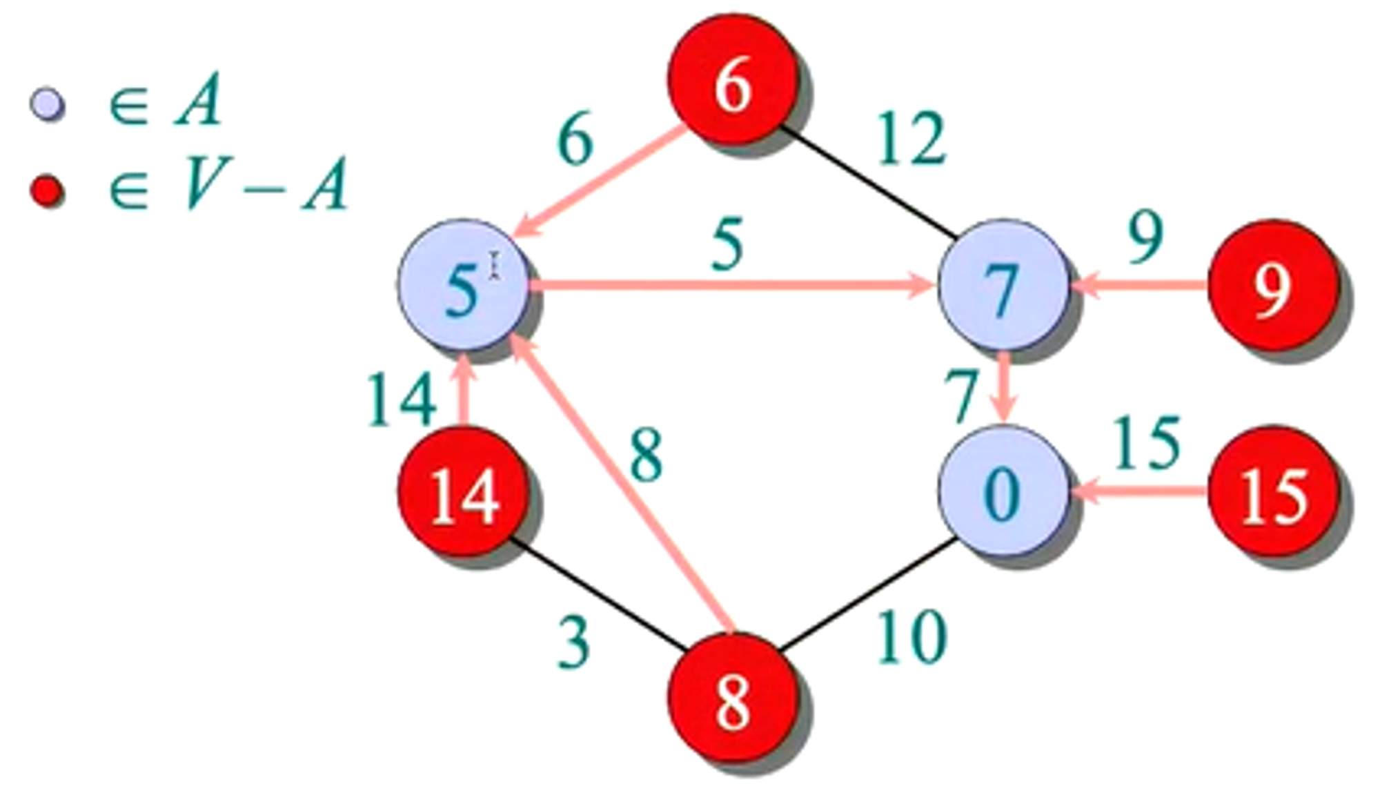
- Choose the next vertex with highest priority.
- Update weights - notice 12→6, 10→8 - even though relaxed once, can be relaxed further
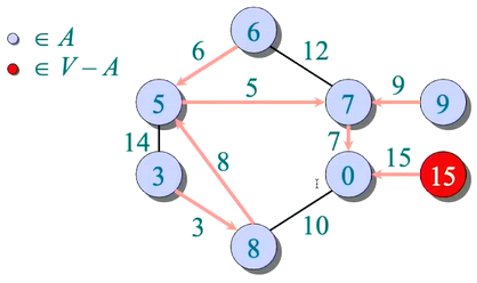
- Choose next vertex with highest priority
- Update weights of adjacent vertices.

1.1.4 - Performance of Prim’s Algorithm
Q <- V
key[v] <- ∞ for all v ∈ V
key[s] <- 0 for some arbitrary s ∈ V
while Q ≠ ∅:
	do u <- extract_min(Q)
		for each v ∈ Adj[u]
			do if v ∈ Q and w(u, v) < key[v]
				then key[v] <- w(u, v)
					π[v] <- u
- We know that the initialisation process (lines 1-3) take time:
- Insertion of all of the vertices in the priority queue can be completed in time if inserted intelligently - all of our start vertices have a priority of except for our start vertex so inserting the start vertex intelligently is all it takes to achieve time.
- Additionally, the two for loops can similarly be completed in time.
- The outermost while loop is executed times, as each vertex is removed from the queue once.
- This also means that we perform extract_min(Q) operations (in time)
- The for-loop iterates at most times, which is the amount of vertices adjacent to it.
- We perform some constant-time operations (i.e. checks in if statement) and may optionally perform a decrease-key operation of time
- Through the handshaking lemma, we know that we’re implicitly performing decrease-key operations
-
Ultimately, the performance of the algorithm depends on the implementation of the priority queue.
PQ Implementation Total unsorted array binary heap fibonacci heap amortised $O(1) $ amortised worst case as
Since as the graph is connected, we can write
-
Fibonacci heaps are very complicated data structures to implement, and have large associated constant factors such that in practice it isn’t really used.