1.0 - Minimum Spanning Tree Algorithms

1.1 - Prim’s Approach

🌱 Look in previous lecture for notes.

1.2 - Kruskal’s Approach

🌱 Initially create a graph with $|V|$ forests (each vertex is a forest) and add least-cost edges that merge forests together. At each step, we perform a locally optimal, greedy action such that it produces a globally optimal solution

T is always a spanning acyclic subgraph; A forest of trees

Initially, T contains all vertices G.V but no edges.
At each step, the least-weighted edge that connects any two trees in the forest T is added to T.
The algorithm stops when T is connected.

1.2.1 - Disjoint Set Data Structure

🌱 To use Kruskal’s algorithm, we need to create a Disjoint Set data structure

The trees in T form disjoint sets of G.V

A disjoint-set data structure maintains a collection $S=\{S_1, S_2, \cdots S_k\}$ $S = {S_{1}, S_{2}, \dots S_{k}}$ of disjoint dynamic sets.
- Disjoint Each element is only in one set
- Dynamic Constantly changing, in that we are merging sets together
Operations are avilable to
- make_set(x) Add a new set that contains element x. Requires that x is not a member of another set
- find_set(x) Returns the representative element for the set containing x.
- union(x, y) Merge the set that contains x with the set that contains y. Uses the link(x, y) subroutine

1.2.2 - Disjoint-Set Implementation as Disjoint-Set Forests

The sets are represented by rooted trees
- Rooted trees tree where the root has a singled-out node as the root
The root of each tree is it’s representative element
Each element x stores:
- x.p The parent of x in its tree (or itself if it is the root - we use this property to identify the root node)
- x.rank An upper bound on the hight of x in this tree - this is important, as our time complexities are dependent on the height of the tree. Storing this allows us to take actions that minimise the height of the tree.

1.2.3 - Operation Analysis

🌱 The make_set(x) method runs in $\Theta(1)$ time.

The make_set(x) method is constant-time as all we need to do is construct a tree containing the element x, and only the element x
In doing this, we set its root node to itself (to designate it as the representative element of this set) and set its rank to 0.

make_set(x):
		# Set x to be its own parent
		x.p = x
		# Set rank (height) of node to 0
		x.rank 0

🌱 The find_set(x) method runs in $\Theta(\log n)$ worst case, and $\Theta(1)$ time typically.

The find_set(x) method returns the top node in the set
- This node is the identifier (representative element) in the set
- It is the only node whose parent is itself.
It applies a path compression heuristic which flattens the tree by setting each node’s parent to representative element

find_set(x):
		# not representative element
		if x ≠ x.p 
				# set current node's parent 
				# to representative element
				x.p = find_set(x.p)
		return x.p # if x = x.p

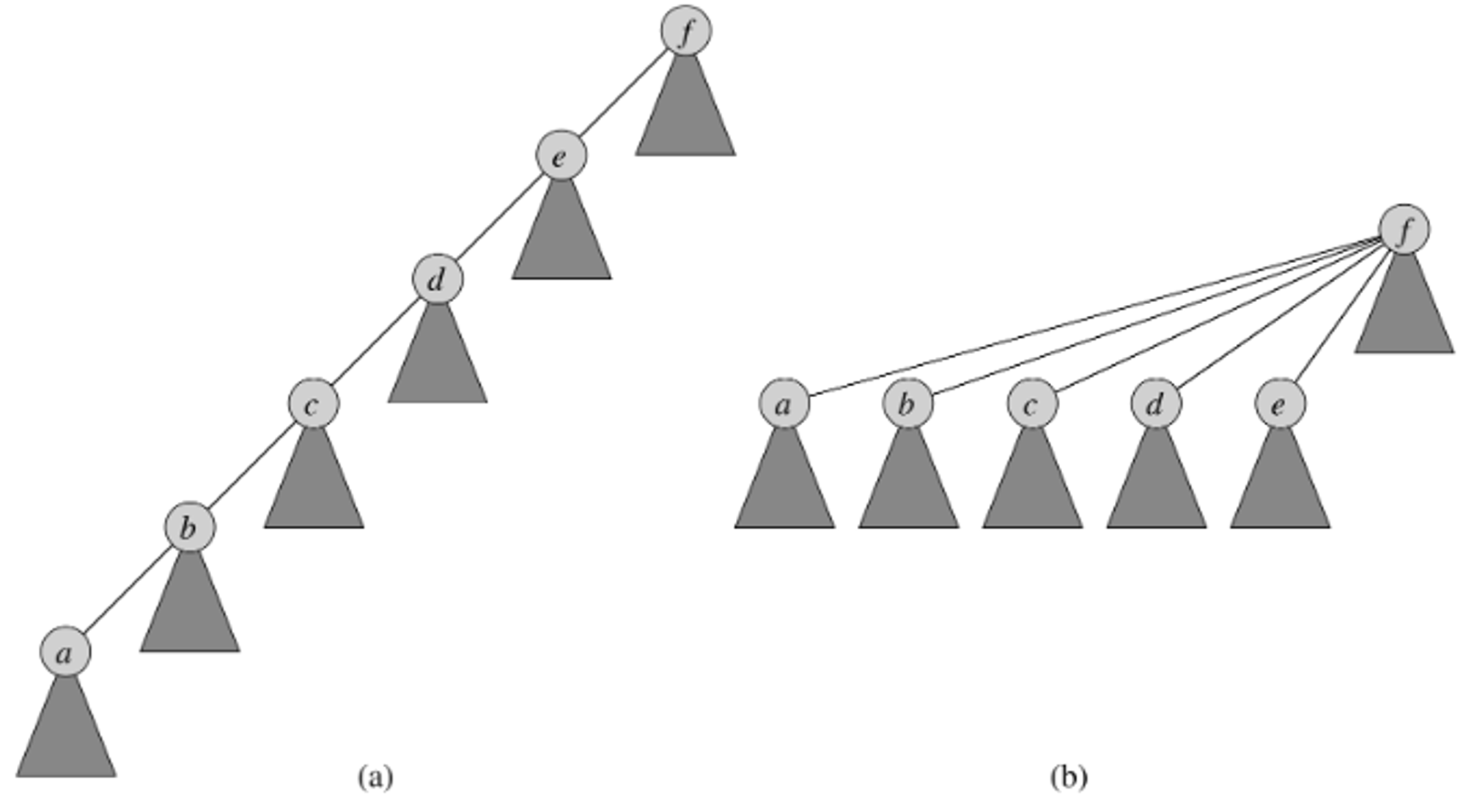
As it traverses the parent links, it collapses them, making them point directly to the top node - this transforms the disjoint forest tree from the left-most figure to the rightmost figure
- Observe that $f$ is still the root node (representative element) and all of the others’ parent nodes have been updated.

🌱 The union(x,y) method merges the two sets that contain x and y into a single tree.

The union(x,y) method merges the sub-trees that contain elements x and y into a single tree, in which its height is guaranteed to be less than or equal to $\log n$ .
It utilises the link subroutine
- In this, we want to link trees in an intelligent manner, to minimise the height of the tree
- If the height of the two trees are equal, we arbitrarily choose one as the parent, and increment the rank of new root node to account for new growth

link(x,y)
		if x.rank > y.rank
			# Set the parent of the shorter tree's
      # root node to taller tree's root node.
			y.p = x 
		else
			x.p = y
			# If the ranks are equal, choose y 
			# as parent, and increment y's rank.
			if x.rank == y.rank
					y.rank = y.rank + 1
union(x,y)
    link(find_set(x), find_set(y))

It applies a rank-by-union heuristic - trees with fewer nodes is made to point to the tree with more nodes
Runs in ‘almost $\Theta(1)$ ’ time - $\Theta(\alpha(n))$ time where $\alpha(n)$ is the inverse Ackermann function which grows extremely slowly.
The rank of a node is determined by the maximum rank of its children (if any), incremented by one.
- $\text{rank}_a=\max(0,0)+1=1$
- $\text{rank}_f=\max(0)+1=1$
- $\text{rank}_e=1$ as leaf node
- $\text{rank}_d=\max(0,1)+1=2$

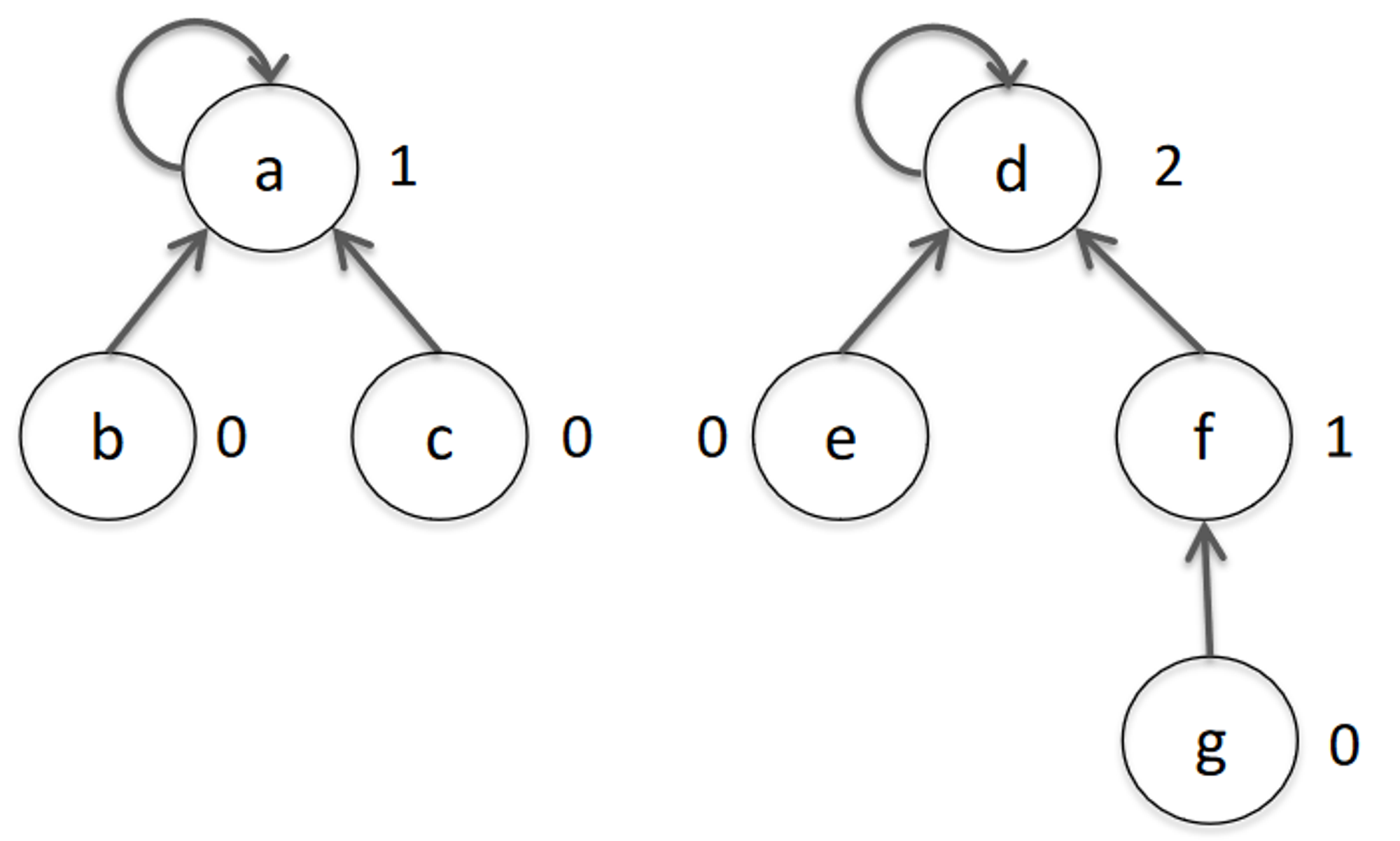
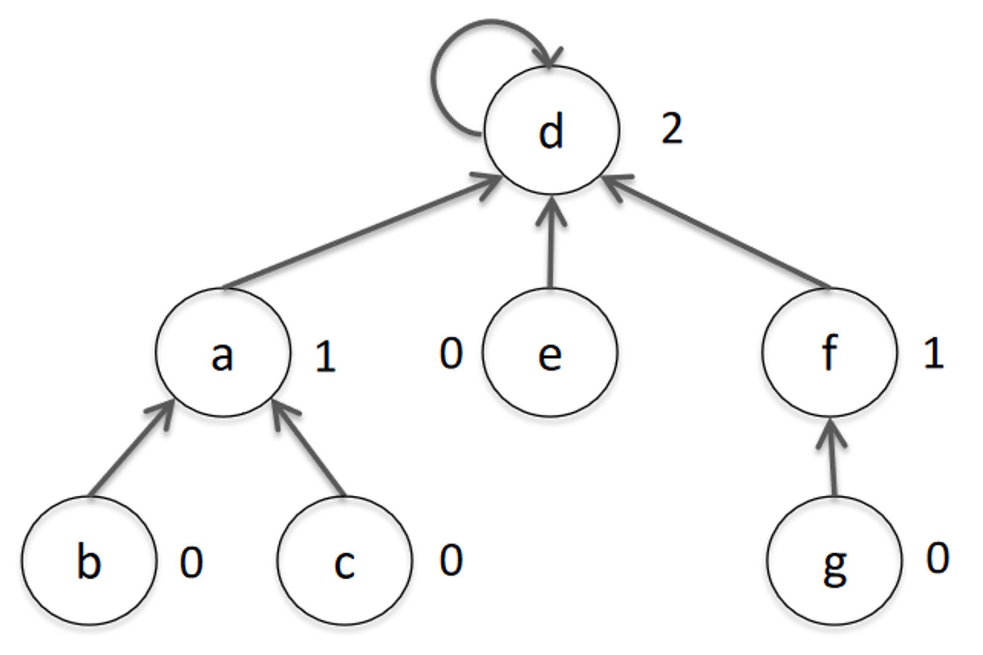
In merging the two (above) forests together, we want to do it in such a way that it minimises the height of the tree (as our time complexity is bounded by the height of the tree).
Therefore, we add the root node of the smaller tree as a child of the root node of the larger tree.

Algorithmically, we represent this as follows
```
mst_kruskal(G, w): # Graph, weights
		T = ∅
		for each vertex v ∈ G.V
				make_set(v)
		sort the edges of G.E into non-decreasing order by weight w
		for each (u, v) taken from the sorted list
				if find_set(u) ≠ find_set(v)
						# Add edge (u, v) to MST subset if 
						# u and v are in different forests.
						T = T ∪ {(u, v)} 
						union(u, v)
		return T
```
- The make_set(v) method takes $\Theta(1)$ time, and is performed $|V|$ times so initialisation takes $\Theta(V)$ time.
- Sorting takes $\Theta(E \lg E)$ time
- The for-loop is run $|E|$ $∣ E ∣$ times, once for each edge.
  - In the for-loop, call find_set four times - this is $O(\lg E)$
  - The total time complexity of the for loop is $O(E \lg E)$
- In total, the time complexity of Kruskal’s algorithm using the disjoint-set forest data structure implementation is $\Theta(E \lg E)$

1.2.4 - Example of Kruskal’s Algorithm

First begin with the start vertex A, and add all of the vertices into the disjoint-set data structure.
At this point, no vertices are connected, and there are $|V|$ forests in the graph T.
We then choose the weight with the lowest cost that connects two forests together - in this case, edge $(g, h)$ has a cost of 1 so we add it to our MST graph.
In doing this, we merge the forest containing $g$ with the forest containing $h$ in our disjoint set data structure

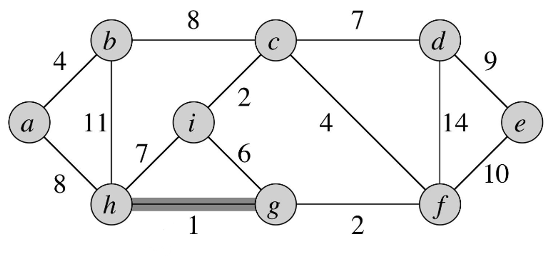
We choose the next edge with the lowest cost and add it to our MST graph, being the edge $(c, i)$
In doing this, we merge the forest containing $i$ with the forest containing $c$ in our disjoint set data structure.

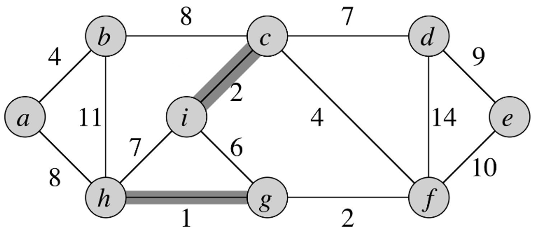
We choose the vertex with the next lowest cost that connects two forest together - in this case, edge $(f, g)$ .
We add this to our MST graph.

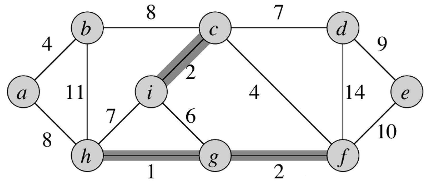
We choose the vertex with the next lowest cost that connects two forests together - in this case, edge $(a, b)$
We add this to our graph.

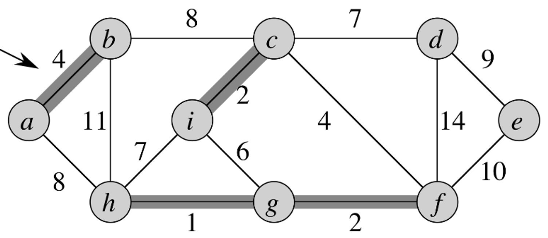
We choose the next vertex with the next lowest cost that connects two forests together - in this case, edge $(c, f)$
We add this to our MST graph.
Observe that this requires the joining of the disjoint sets $\{\{c, i\}, \{f, g, h\}\}$

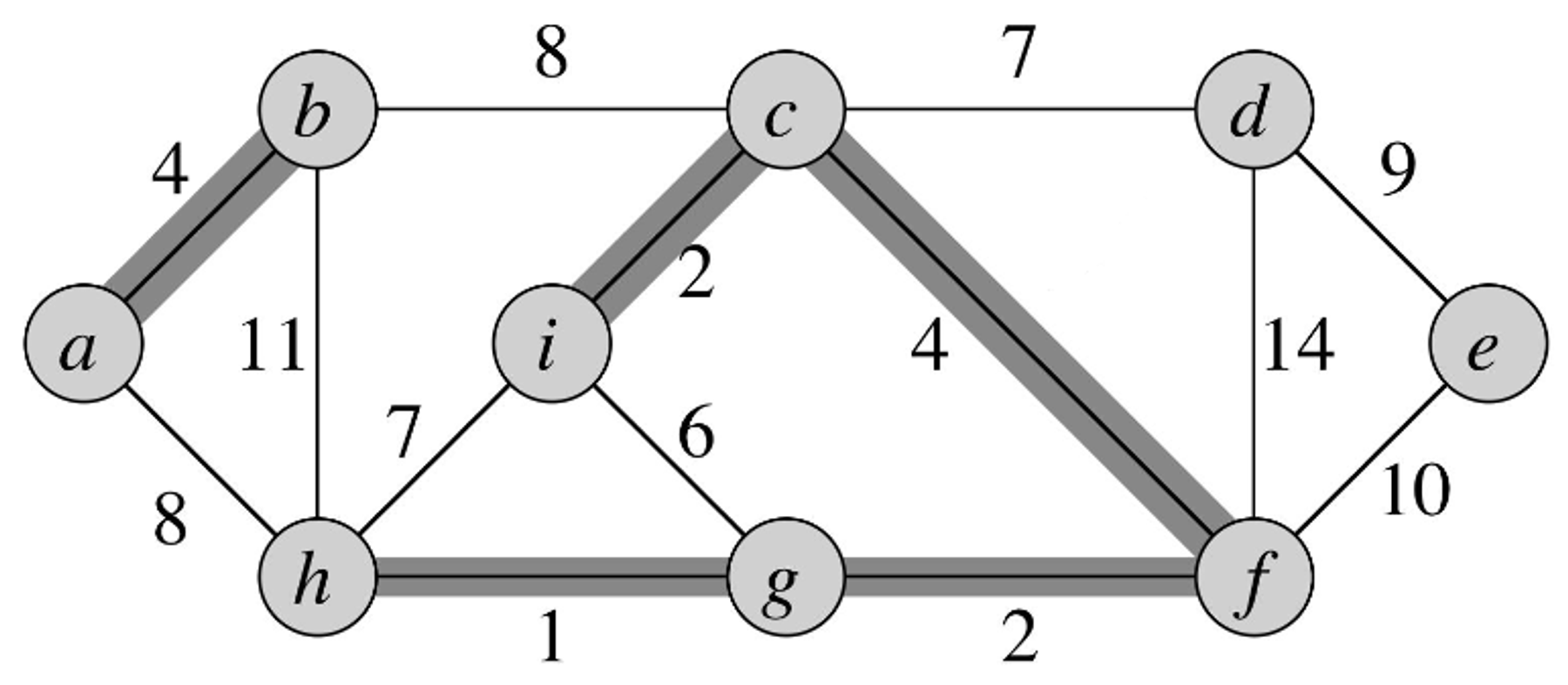
Here, the edge with the next lowest cost is $(i, g)$ but it doesn’t conect two forests together, so we don’t add it to our graph
We continue with our search, evaluating the next edge.

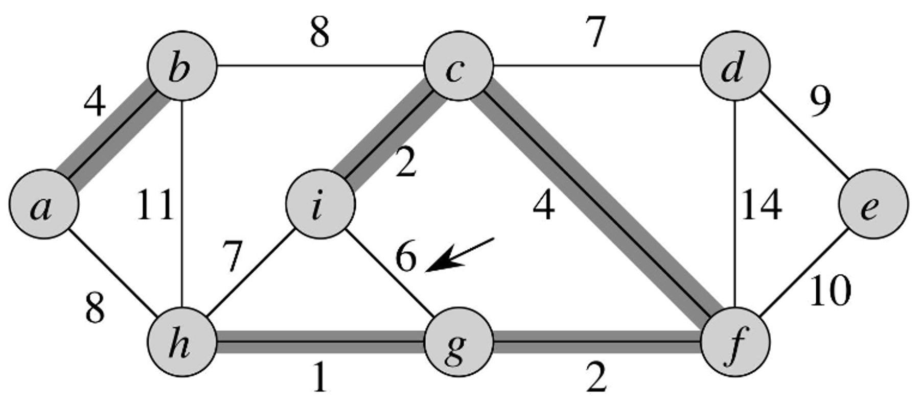
Here, we add the edge $(c,d)$ as it connects two disjoint forests.
We add this to our MST graph.

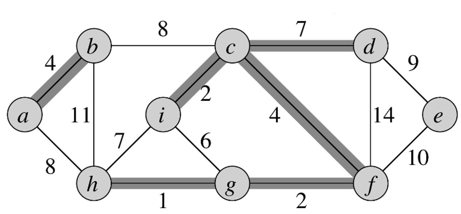
The edge with the next lowest cost is $(h, i)$ but it doesn’t connect two disjoint forests so we don’t add it to our MST graph being constructed.

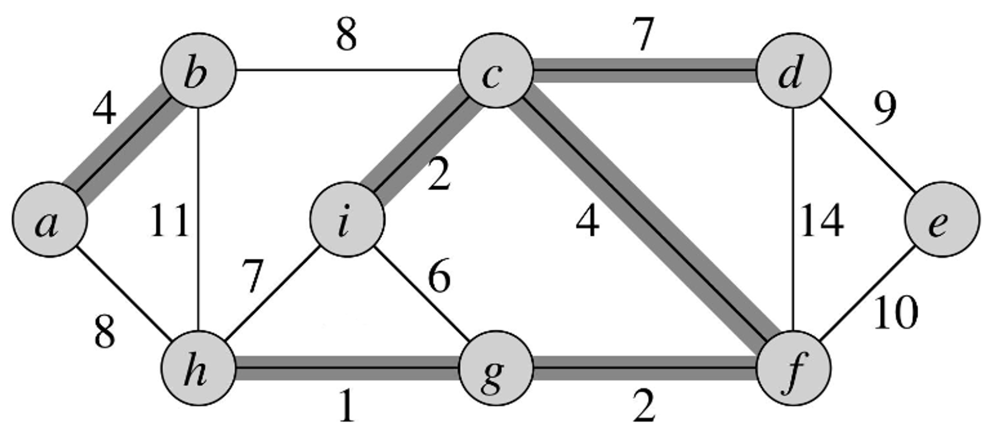
The next edge with the lowest cost is $(a, h)$ and it connects two disjoint forests, so we add it to the MST graph being constructed.

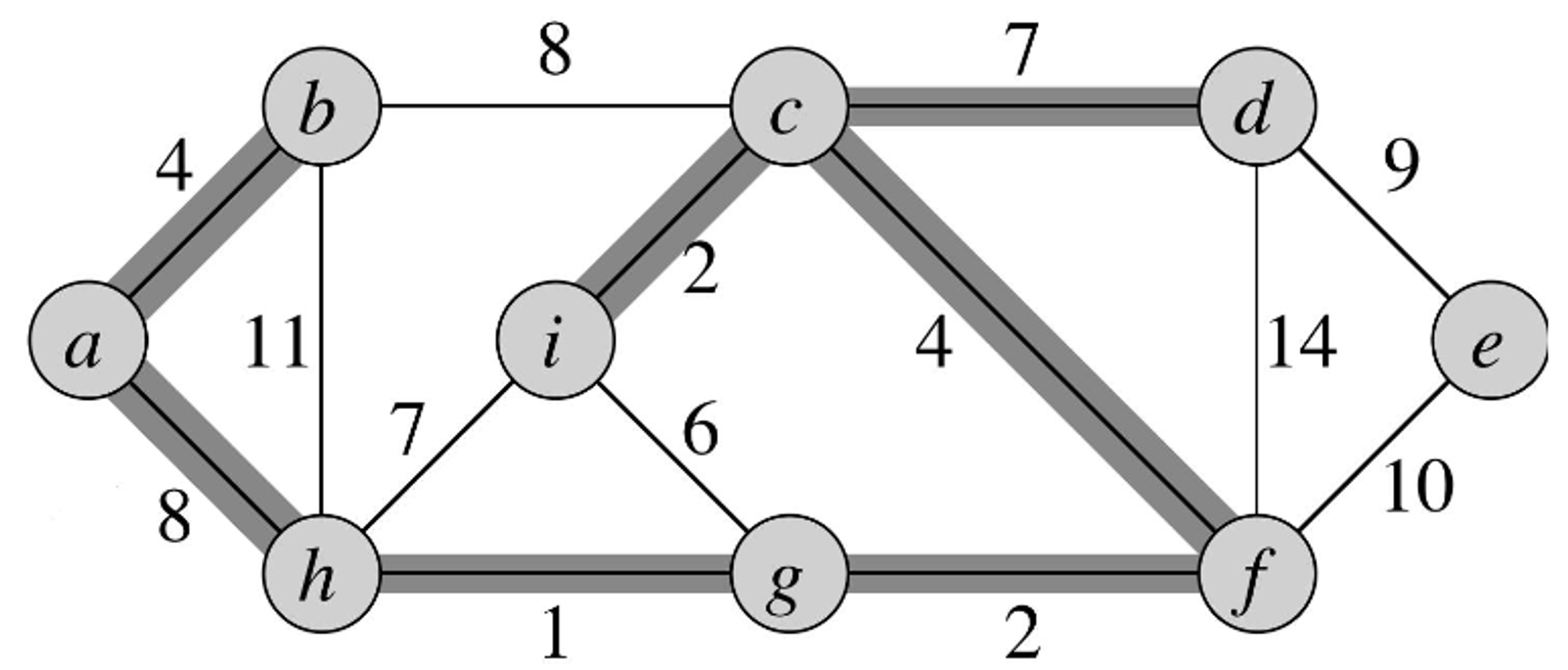
The next edge with the lowest cost is $(b, c)$ but it doesn’t connect any disjoint forests so we don’t add it to the MST being constructed.

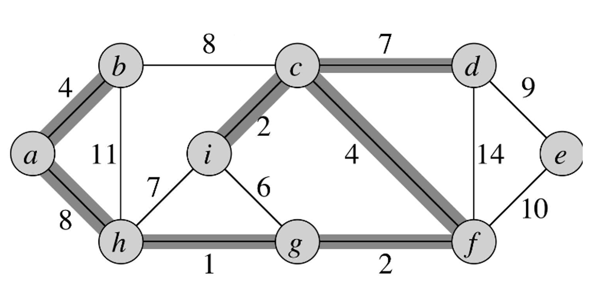
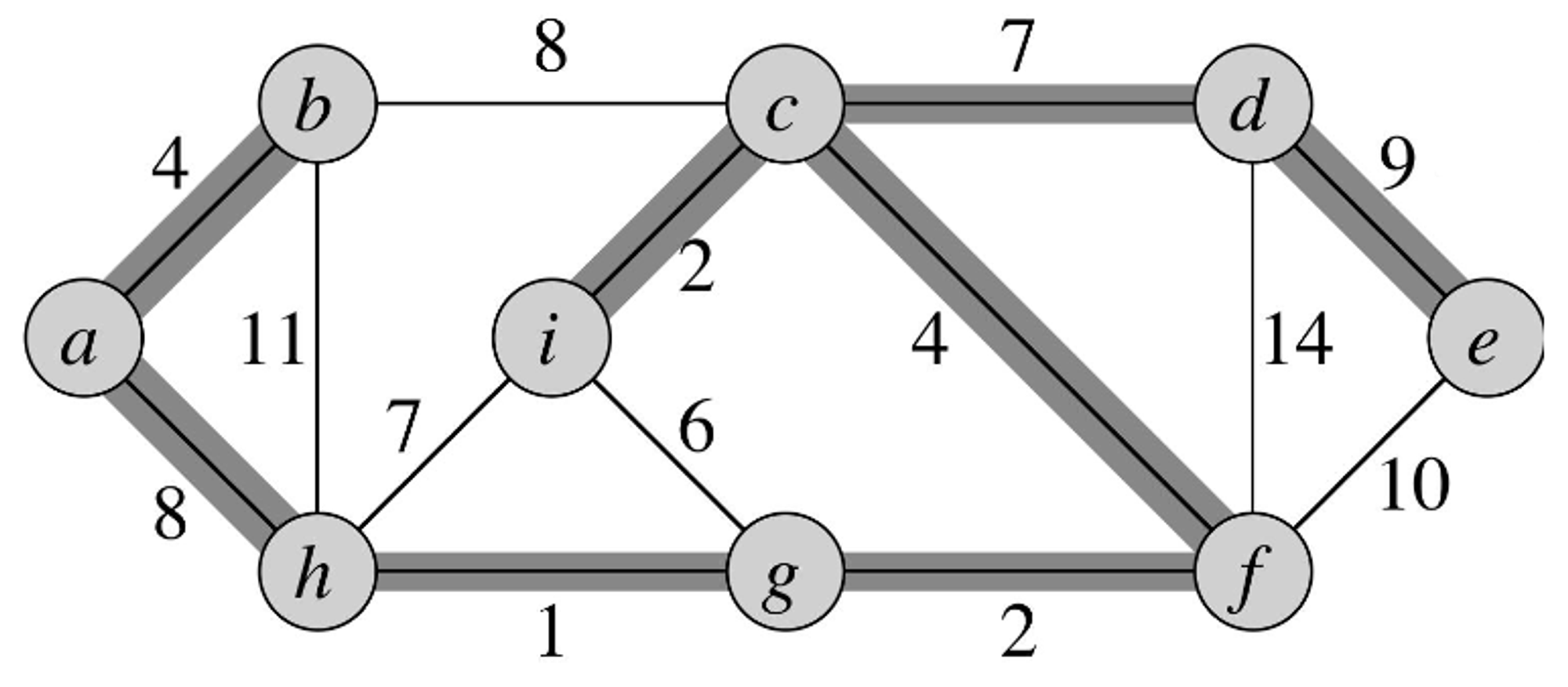
- The next edge with the lowest cost is $(d, e)$ which connects two disjoint forests so we add it to the MST being constructed.

The next edge with the lowest cost is $(b, h)$ but it doesn’t connect any disjoint forests so we don’t add it to the MST being constructed.

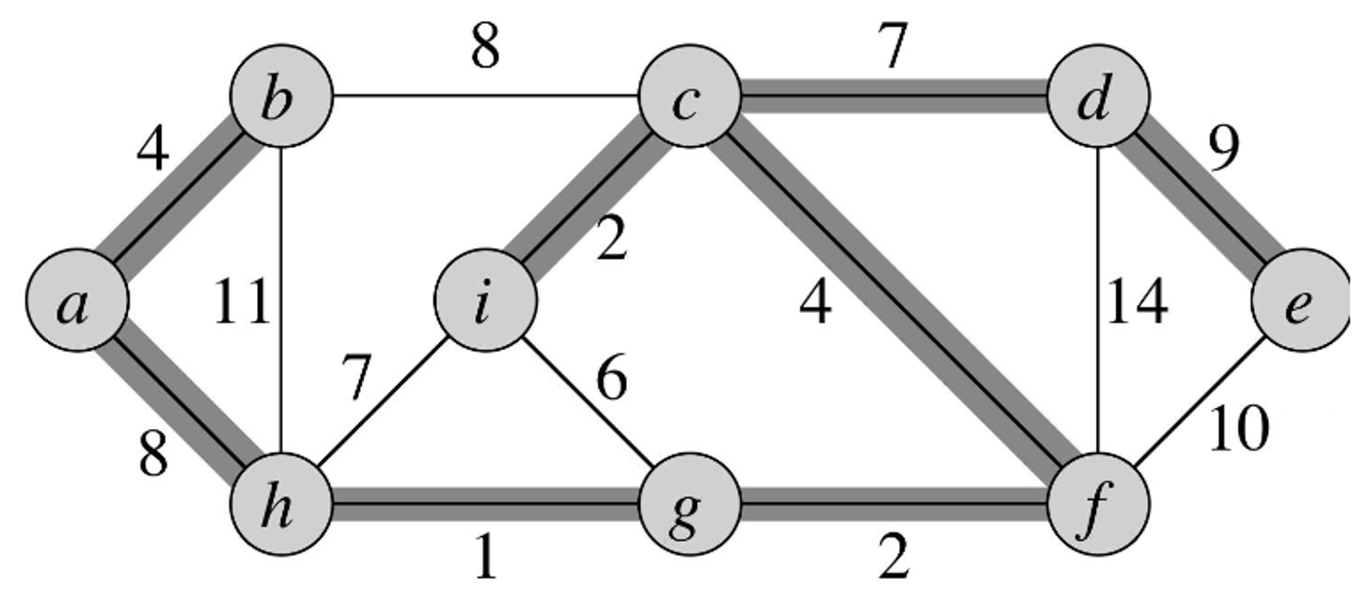
Finally, the edge with the highest cost is $(d, f)$ but it doesn’t connect any disjoint trees.
At the end of this process, we have constructed the MST for this graph.