1.0 - Dynamic Programming

🌱 Using Dynamic Programming, we can cause massive speed improvements: from exponential-time to polynomial time

A method for efficiently solving problems of a certain kind, by storing the results to sub-problems.
May apply to problems with optimal sub-structure.
An optimal solution to a problem can be expressed (recursively) in terms of optimal solutions to sub-problems of the same kind.
A naïve recursive solution may be inefficient (exponential) due to repeated computations of sub-problems
Dynamic programming avoid re-computation of sub-problems by storing them.
Requires a deep understanding of the problem and its solution, however some standard formats apply.

🌱 Problems can have different optimal sub-structures, that impact the efficiency of the final solution

Dynamic programming constructs a solution “bottom-up”
- We need to compute solutions to base-case sub-problems first
- Then methodically calculate all intervening sub-problems;
- Until the required problem can be computed

1.1 - Memoisation

Memoisation is a type of dynamic programming (i.e. solutions to sub-problems are stored so that they are never recomputed)
It is top-down in the same sense as recursion
It is often more “elegant’ but has slightly worse constant factors associated as a result of the recursive calls (rather than the iterative approach)

1.2 - Fibonacci using Dynamic Programming

🌱 Many problems are naturally expressed recursively. However, recursion can be computationally expensive.

Fibonacci numbers can be defined using the following formula:

$F(i)=\begin{cases}1&\text{if i=1 or i=2}\\F(i-1)+F(i-2)& \text{otherwise}\end{cases}$
That is, we can express a larger problem as a combination of smaller problems.

As a result of this, we have a simple recursive expression for computing Fibonacci numbers

Fibonacci(n)
    if n == 1 or n == 2:
        return 1
    else
				return Fibonacci(n-1) + Fibonacci(n-2)

The recurrence describing the performance of this algorithm is given as:

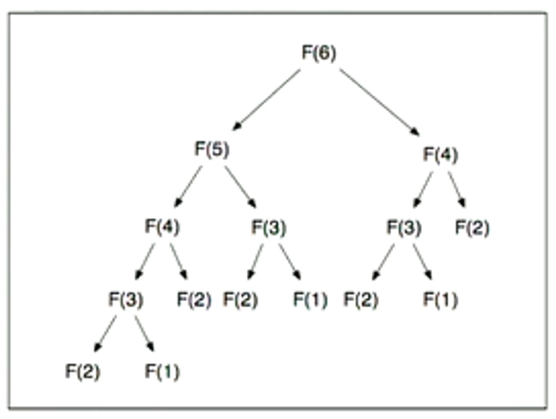
$\begin{aligned}T(n)&=T(n-1)+T(n-2)+\Theta(1)\\&\approx\Theta(1.6^n)\end{aligned}$
The time complexity of this recurrence is terrible, as we’re performing a lot of recomputing.
F(3) = 3
F(2) = 5

Instead of recalculating a number that we’ve already seen, store the original calculation in an array, and look it up when encountered later.

In our dynamic solution to the Fibonacci problem, we use an array to store our previous computations

fibonacci_dynamic(n)
    T = new int[n]
    T[1] = 1
    T[2] = 1
    for i = 3..n
       T[i] = T[i-1] + T[i-2]
    return T[n]

The elements in the array correspond to the mathematical definition
The time complexity analysis of the dynamic Fibonacci algorithm:

$T(n)=\sum^n_{i=3} \Theta(1) \in \Theta(n)$
Additionally, this algorithm consumes $\Theta(n)$ space, as we construct an auxiliary data structure in an array of size $n$
- However, we can reduce this space complexity by only storing the previous two calculations

We can also construct a memoised Fibonacci algorithm

Assume that array T is a global variable, and we will never require a Fibonacci number past N

fibonacci_init()
    T = new int[N]
    for i = 1..N
				T[i] = null
    T[1] = 1
    T[2] = 1

fibonacci_memoised(n)
    if T[n] == null // Check if we have already computed a solution
         T[n] = fibonacci_memoised(n-1) + fibonacci_memoised(n-2)
    return T[n]

This will have slightly worse constant factors than the bottom-up approach as a result of the recursive calls made.

1.3 - Solving Problems using Dynamic Programming

🌱 Solving problems using recursion is often intuitive and elegant, however it can be massively inefficient.

If:

The problem has the optimal substructure property, and
It’s recursive solution has overlapping sub-problems,

Then dynamic programming techniques may apply. Doing this, we get an efficient (polynomial-time) implementation for the loss of elegance.

1.4 - Longest Common Subsequence (LCS)

🌱 Find the longest (non-contiguous) sequence of characters shared between two strings

The longest (non-contiguous) sequence of characters shared between the following two strings are:

$\def\t{\ \ \ \ } S_1: {\color{lightblue}A}\t {\color{lightblue}B}\t C\t {\color{lightblue}B}\t C\\ S_2: C\t {\color{lightblue}A}\t {\color{lightblue}B}\t {\color{lightblue}B}\t D\\ LCS(S_1, S_2)=ABB$
Assuming that you have already solved any strictly smaller subproblem(s).
How can you use that to solve your top-level problem?
- We need to identify the base cases.

1.4.1 - Determine Base Cases

Suppose that we have calculated the LCS for $S_1=ABCBC, S_2=CABBD$
- $LCS(S_1,S_2)=ABB$
What is the LCS of $S_1=ABCBCE, S_2=CABBDE$ ?
- More clearly, what is the LCS of $S_1\cdot E$ and $S_2\cdot E$ where $\cdot$ denotes string concatenation
- Thus, $LCS(S_1\cdot E, S_2\cdot E)=LCS(S_1,S_2)\cdot E$
Consider LCS of $S_3=ABCBCX$ and $S_4=CABBDY$
That is, $S_1\cdot X$ and $S_2\cdot Y$ where $X\ne Y$ it is possible that X is in $S_2$ or Y is in $S_1$
That is, we consider when $X\ne Y$ , we recursively look at both possibilities and chose the maximum

$LCS(S_1\cdot X, S_2\cdot Y)=\max(LCS(S_1\cdot X, S_2), LCS(S_1, S_2\cdot Y))$
- This is a sub-problem, as in either case, we are throwing away a character (making the problem smaller)
We have now considered the cases for $S_1\cdot X$ and $S_2\cdot X$ where $X=Y$ and $X\ne Y$ .
Using this, we can construct our base cases together:

$\begin{aligned} \text{LCS}(\langle\rangle, S_2) &=\ \text{LCS}(S_1, \langle \rangle)=\langle \rangle\\ \text{LCS}(S_1\cdot X, S_2\cdot X)&=\text{LCS}(S_1, S_2)\cdot X\\ \text{LCS}(S_1\cdot X, S_2\cdot Y)&=\max(\text{LCS}(S_1, S_2\cdot Y), \text{LCS}(S_1\cdot X, S_2)\ \ \ \ \text{when } X\ne Y \end{aligned}$

1.4.2 - Implementing Length of LCS Algorithm

Using the base cases identified above, we can implement an algorithm which determines the length of two strings’ LCS.

$\def\lcs{\text{LCS}} \begin{aligned} \lcs(\langle\rangle, S_2)&=\lcs(S_1, \langle\rangle)=0\\ \lcs(S_1\cdot X, S_2\cdot X)&=\lcs(S_1, S_2)+1\\ \lcs(S_1\cdot X, S_2\cdot Y)&=\max(\lcs(S_1, S_2\cdot Y), \lcs(S_1\cdot X, S_2))\ \ \ \text{when } X\ne Y \end{aligned}$

1.4.3 - Recursive, Non-Dynamic Implementation

We will use a recursive implementation using arrays and indexes.

We initially call lcs_length_rec($S_1, S_2, n, m)$ where

$\text{length}(S_1)=n$ and $\text{length}(S_2)=m$ (in which we index from 1)
n and m specify the length of the LCS we are computing

lcs_length_rec(S1, S2, i, j)
    if i == 0 or j == 0
				// base case
        return 0
    else 
        if S1[i] == S2[j]:
            return lcs_length_rec(S1, S2, i-1, j-1) + 1
        else
            return max(
                       lcs_length_rec(S1, S2, i-1, j), // Reduce S1
                       lcs_length_rec(S1, S2, i, j-1)
                      )

We can characterise the performance of this algorithm as:

$\scriptsize T(i, j)=\begin{cases}\Theta(1)&\text{when } i=0 \text{ or }j=0\\ T(i-1, j)+T(i,j-1)+\Theta(1)&\text{when } i>0 \text{ or } j > 0\end{cases}$
The running time of this algorithm is exponential, as there are $\Omega(2^{\min(n,m)})$ possible sub-sequences to check
We have solved an optimisation problem by finding optimal solutions to subproblems.
A quick inspection confirms that there will be overlapping subproblems, and hence extreme inefficiency for this recursive implementation.
How many sub-problems are there when $\text{length}(S_1)=n$ and $\text{length}(S_2)=m$ when indexing from 1

$(n+1)\times(m+1)$

1.4.4 - Recursive, Dynamic Implementation

Note here that the order in which we compute the problems is important.
Here, our subproblems either have a lower value of i, a lower value of j, or both

lcs_length_dyn(S1, S2, n, m)
    T = new int[n+1][m+1]
    // Insert base cases into the table
    for i = 1 to n
        T[i,0] = 0
    for j = 1 to m
        T[0,j] = 0
    for i = 1 to n
        for j = 1 to m
            if S1[i] == S2[j]
                T[i,j] = T[i-1, j-1] + 1
            else if T[i-1, j] > T[i, j-1]
                T[i,j] = T[i-1, j]
            else 
                T[i,j] = T[i, j-1]

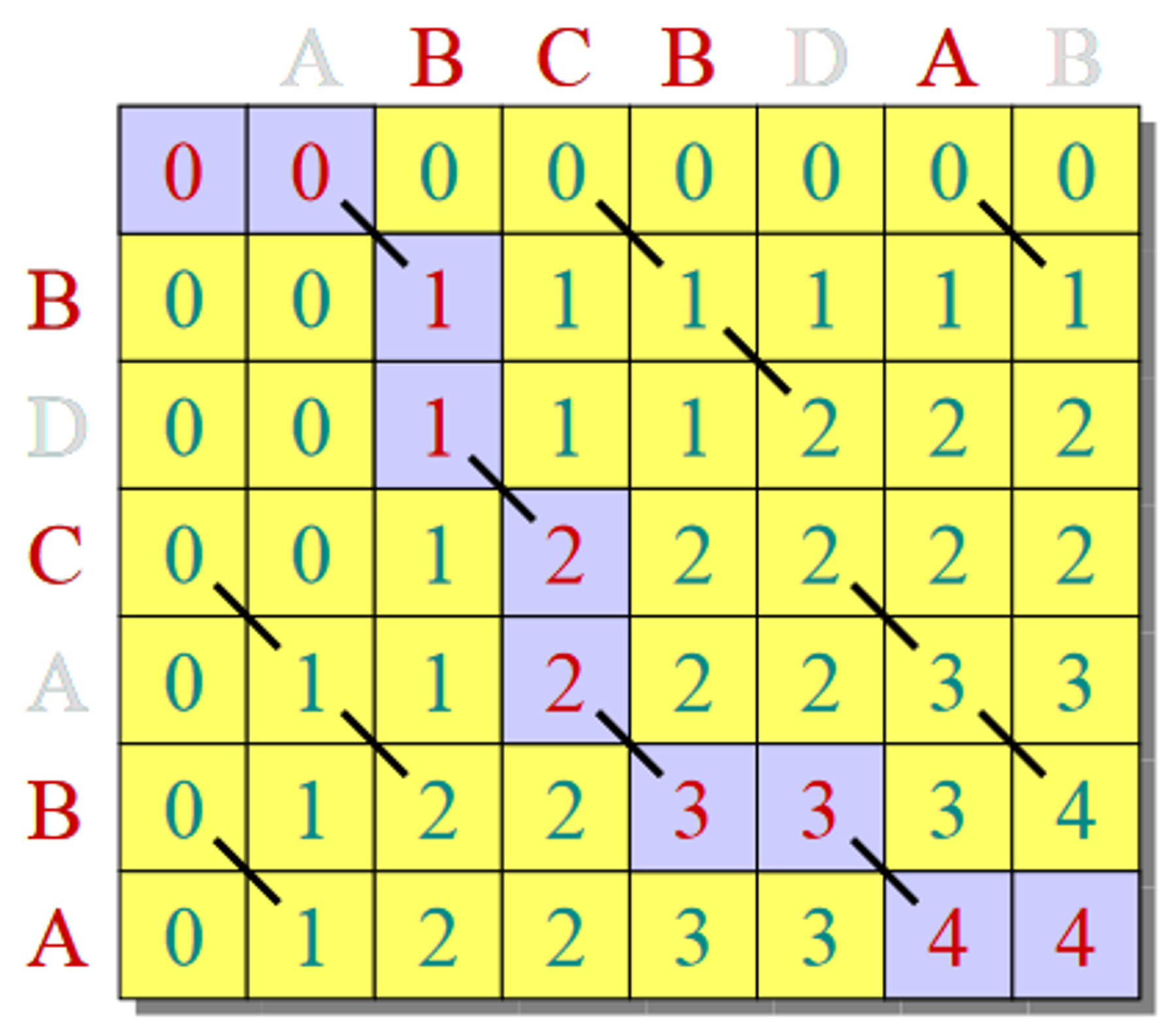
This problem has $T(n)\in\Theta(n\times m)$ time complexity.

1.4.5 - Reconstructing the Path

We can construct the LCS table bottom-up in $\Theta(mn)$ time.
If we remember the decisions that we made at each time step, we can reconstruct the LCS by tracing this path backward.