Lindholm Chapter 10 - Generative Models and Unlabelled Data

Gaussian Mixture Model and Discriminant Analysis.

• The Gaussian Mixture Model makes use of the factorisation of the joint PDF

$$p({\bf x}, y) = p({\bf x} | y) p(y) \tag{10.1a}$$

• The second factor is the marginal distribution of $y$.
• Since $y$ is categorical and thereby takes values in the set $\lbrace 1, \dots, M \rbrace$, this is given by a categorical distribution with $M$ parameters, $\lbrace \pi_m \rbrace_{m=1}^M$.

$$p(y=1) = \pi_1 \\ \vdots \\ p(y=M) = \pi_M \tag{10.1b}$$

• The first factor in Equation 10.1a is the class-conditional distribution of the input $\bf x$ for a certain class $y$. In a classification setting, it is natural to assume that these distributions are different for different classes of $y$.
• If it is possible to predict the class $y$ based on the information in $\bf x$ then the characteristics (distribution) of $\bf x$ should depend on $y$.
• Need to make further assumptions on these class-conditional distributions.
• The basic assumption for a GMM is that each $p({\bf x} | y)$ is a Gaussian Distribution with a class-dependent mean vector ${\boldsymbol \mu}_y$ and covariance matrix ${\boldsymbol \Sigma}_y$.

$$p({\bf x} | y) = \mathcal{N}({\bf x} | {\boldsymbol \mu}_y, {\bf \Sigma}_y) \tag{10.2}$$

Supervised Learning of the Gaussian Mixture Model

• The unknown parameters to be learned are $\theta=\lbrace {\boldsymbol\mu}_m, {\boldsymbol\Sigma}_m, {\boldsymbol\pi}_m\rbrace_{m=1}^M$.
• Start with the supervised case, meaning that the training data contains inputs $\bf x$, and corresponding outputs $y$ - $\mathcal{T}=\lbrace{\bf x}_i, y_i \rbrace_{i=1}^n$.
• Mathematically we learn the GMM by maximising the log-likelihood of the training data:

$$\hat\theta=\arg\max_\theta \ln p(\underbrace{\lbrace {\bf x}_i, y_i \rbrace_{i=1}^n}_{\mathcal{T}} | \theta) \tag{10.2a}$$

• Due to the generative model, this is based on the joint likelihood of the inputs and outputs.
• From this, we derive the model definition is given by:

$$\begin{align*} \ln p (\lbrace {\bf x}_i, y_i \rbrace_{i=1}^n |\theta) &= \sum_{i=1}^n \lbrace \ln p({\bf x}_i | y_i, \theta) + \ln p(y_i | \theta) \rbrace \\ &= \sum_{i=1}^{n} \sum_{m=1}^M \mathbb{I} \lbrace y_i = m \rbrace \left \lbrace \ln \mathcal{N} ({\bf x}_i | {\bf \mu}_m, {\bf\Sigma}_m) + \ln \pi_m \right \rbrace \tag{10.2b} \end{align*}$$

• The indicator function effectively separates the log-likelihood function into $M$ independent sums - one for each class
  • Separates based on the class labels of the training points.
• The optimisation problem has a close-form solution.
• Begin with marginal class probabilities, $\lbrace \pi_m \rbrace_{m=1}^M$, where $n_m$ is the number of training points in class $m$.
  • Therefore $\sum_m n_m = n$ and thus $\sum_m \hat\pi_m = 1$.

$$\hat\pi_m =\frac{n_m}{n} \tag{10.3a}$$

• The mean vector ${\bf\mu}_m$ of each class is estimated as:

$${\bf\mu}_m = \frac{1}{n_m} \sum{i: y_i = m} ({\bf x}_i - \hat{\bf\mu}_m)({\bf x}_i - \hat{\bf\mu}_m)^T\tag{10.3c}$$

• The equations 10.3b and 10.3c learns a Gaussian distribution for $\bf x$ for each class such that the mean and covariance matching.
  • Note that $\hat\theta$ can be computed regardless of whether the data really comes from a Gaussian distribution or not.

Predicting Output Labels for New Inputs: Discriminant Analysis

• The key insight for using generative model $p({\bf x}, y)$ to make predictions is to realise that predicting the output $y$ for a know value $\bf x$ amounts to computing the conditional distribution $p(y|{\bf x})$:

$$\def\x{{\bf x}} p(y|\x) = \frac{p(\x, y)}{p(\x)} = \frac{p(\x, y)}{\sum_{j=1}^M p(\x,y=j)}\tag{10.4}$$

• From this, we get the classifier:

$$p(y=m |{\bf x_\star}) = \frac{ \hat\pi_m \mathcal{N}\left({\bf x_\star} | \hat{\bf\mu}_m, \hat{\bf\Sigma}_m \right) } { \sum_{j=1}^M \hat\pi_j \mathcal{N}\left( {\bf x_\star} | \hat{\bf\mu}_j, \hat{\bf\Sigma}_j\right) }\tag{10.5}$$

• We obtain the hard predictions $\hat y_\star$ by selecting the class with the highest probability prediction

$$\hat y_\star = \arg\max_m p(y=m | {\bf x_\star}) \tag{10.6}$$

• Taking the logarithm and noting that only the numerator in Equation 10.5 depends on $m$, we can equivalently write:

$$\hat y_\star = \arg\max_m \left\lbrace \ln \hat\pi_m + \ln \mathcal{N}\left({\bf x_\star} | \hat{\bf\mu}_m, \hat{\bf\Sigma}_m\right) \right \rbrace \tag{10.7}$$

• Since the logarithm of the Gaussian PDF is a quadratic function in $\bf x$, the decision boundary for this classifier is quadratic - this is called Quadratic Discriminant Analysis (QDA).
• If we make an additional simplifying assumption about the model, instead Linear Discriminant Analysis (LDA) is obtained.
  • The simplifying assumption is that the covariance matrix is equal for all classes, i.e. ${\bf\Sigma}_m = {\bf\Sigma}$ for all $m$.
• This new covariance matrix is replaced by the covariance matrix learned by the following equation.
• This simplifying assumption results in a cancellation of a cancellation of all quadratic terms when computing class probabilities, when computing class predictions using Equation 10.7.
  • Consequently, LDA is a linear classifier just like Logistic regression - will often perform similarly.
  • Will not perform identically as parameters are learned in different ways.

$$\hat{\bf\sigma} = \frac 1n \sum_{m=1}^{M} \sum_{i:y_i=m} ({\bf x}_i = \hat{\bf\mu}_m)({\bf x}_i = \hat{\bf\mu}_m)^T \tag{10.8}$$

• The pseudocode for training the GMM is given as:

Data Training data $\mathcal{T} = \lbrace {\bf x}_i, y_i \rbrace_{i=1}^n$.

Result Gaussian Mixture Model

1. for $m=1, \dots, M$ do
2.  |   Compute $\hat\pi_m$ using Equation 10.3a, $\hat{\bf\mu}_m$ using Equation 10.3b and $\hat{\bf\Sigma}$ using Equation 10.3c
3. end

• The pseudocode for predicting using the GMM is given as:

Data Gaussian Mixture Model and test input $\bf x_\star$.

Result Prediction $\hat y_\star$.

1. for $m=1, \dots, M$ do
2.  |   $\delta_m \overset{\text{def}}= \ln\hat{\bf pi}_m + \ln \mathcal{N}\left({\bf x_\star} | \hat{\bf\mu}_m, \hat{\bf\Sigma}_m\right)$.
3. end
4. Set $\hat y_\star = \arg\max_m \delta_m$

Semi-Supervised Learning of the Gaussian Mixture Model

Want to exploit the information available in the unlabelled data to end up with a better model

• Consider semi-supervised learning problem, where some of the output values $y_i$ are missing in the training data.

• The input values ${\bf x}_i$ for which the output is missing are called unlabelled data points.

• Denote the total number of training points as $n$, out of which only $n_l$ are labelled input-output pairs $\lbrace {\bf x}_i, y_i \rbrace_{i=1}^{n_l}$ and the remaining $n_u$ unlabelled data points are $\lbrace {\bf x}_i \rbrace_{i=n_l+1}^{n}$.

  

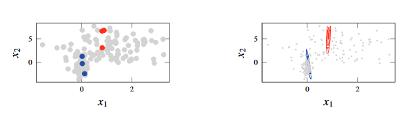
  Figure 1 - Semi-supervised learning, in which which we have fitted a GMM to data in which we do not have most of the labels. The unlabelled data has evidently made the problem harder

• One way to approach a semi-supervised problem is to use a generative model.

• A generative model is a model of the joint distribution $p({\bf x}, y)$ which can be factorised as $p({\bf x}, y) = p({\bf x})p({\bf x}|y)$.

  • Since the marginal distribution of the inputs $p({\bf x})$ is a part of the model, it seems plausible that the unlabelled data can be useful.

• Intuitively, the unlabelled inputs can be used to find groups of input values with similar properties - which are then assumed to be of the same class.

• Use the maximum-likelihood approach - seek model parameters that maximise likelihood of observed data.

$$\hat\theta=\arg\max_\theta \ln p( \underbrace{ \lbrace \lbrace {\bf x}_i, y_i\rbrace_{i=1}^{n_l}, \lbrace {\bf x}_i\rbrace_{i=n_l+1}^{n} \rbrace }_{\mathcal{T}} )$$

• This problem has no closed-form solution.
• When computing the mean vector for the $m$th class we do not know which points should be included in the sum.
• We could first learn an initial GMM which is then used to predict the missing labels.
  • We then use these predictions to update the model.
• This iterative process results in te following algorithm:
  1. Learn the GMM from the $n_l$ labelled input-output pairs
  2. Use the GMM to predict (as a QDA classifier) the missing outputs
  3. Update the GMM including the predicted outputs from step 2
  4. Repeat steps (2) and (3) until convergence
• From Step 2, we should return the predicted class probabilities and not the class predictions predicted using the current parameter estimates
• We make use of the predicted class probabilities using the Equation 10.10a

$$w_i (m) = \begin{cases} p(y=m |{\bf x}_i \hat\theta) & \text{ if } y_i \text{ is missing}\\ 1 & \text{if } y_i=m\\ 0 & \text{otherwise} \end{cases}\tag{10.10a}$$

• We update the parameters using the following equations

$$\begin{align*} \hat\pi_m &= \frac{1}{n} \sum_{i=1}{n} w_i(m) \tag{10.10b}\\ \hat\mu_m &= \frac{1}{\sum_{i=1}^{n} w_i (m)} \sum_{i=1}^{n} w_i(m) {\bf x}_i \tag{10.10c}\\ \hat\Sigma_m &= \frac{1}{\sum_{i=1}^{n} w_i (m)} \sum_{i=1}^{n} w_i(m) ({\bf x}_i - \hat\mu_m) ({\bf x}_i - \hat\mu_m)^T \tag{10.10d} \end{align*}$$

• The pseudocode for the semi-supervised learning of the GMM is given as:

Data: Partially labelled training data $\mathcal{T} = \lbrace\lbrace {\bf x}_i, y_i \rbrace_{i=1}^{n_l}, \lbrace {\bf x}_i \rbrace_{i=n_l+1}^{n}\rbrace$ with output classes $m=1,\dots,M$.

Result Gaussian Mixture Model

1. Compute $\theta=\lbrace \hat{\bf\pi}_m, \hat{\bf\mu}_m, \hat{\bf\Sigma}_m \rbrace_{m=1}^M$ according to Equation 10,3 using only the labelled data
2. repeat
3.  |   For each ${\bf x}_i$ in the unlabelled subset, compute the prediction $p(y|{\bf x}_i, \hat\theta)$ according to Equation 10.5 using the current parameter estimates
4.  |   Update the parameter estimates $\hat\theta=\lbrace \hat{\bf\pi}_m, \hat{\bf\mu}_m, \hat{\bf\Sigma}_m \rbrace_{m=1}^M$ according to Equation 10.10
5. until convergence

• The prediction is done in an identical fashion to QDA (Method 10.1)

Cluster Analysis

• Models in supervised learning have the objective to learn input-output relationship based on examples.

• In semi-supervised learning, mixed labelled and unlabelled data to learn a mode which makes use of both sources of information

• In unsupervised learning assume that all points are unlabelled.

• Objective is to build a model that can be used to reason about key properties of the data (or the process usd to generate the data)

• Clustering is highly related to classification

• Assign a discrete index to each cluster and say all $\bf x$ values in the $m$th cluster are of class $y=m$.

  • Difference between clustering and classification is that we train based on the $\bf x$ values without any labels.

Unsupervised Learning of the Gaussian Mixture Model

• The GMM is a joint model for $\bf x$ and $y$, given by

$$p({\bf x}, y) = p({\bf x} | y) p(y) = \mathcal{N} \left({\bf x} | {\bf\mu}_y, {\bf\Sigma}_y\right) \pi_y \tag{10.11}$$

• To obtain a model for only $\bf x$ we can marginalise out $p({\bf x})=\sum_y p({\bf x}, y)$ from it.
  • That is, we consider $y$ as being a latent random variable - a random variable that exists in the model but is not observed in the data.
• In practice, still lean the joined model, but from data containing only $\bf x$ values.
• We want to learn which ${\bf x}_i$ values come from the same class-conditional distribution$p({\bf x}|y)$ based on their similarity.
  • That is, the latent variables $y$ need to be inferred from this data, and then use this latent data to fit the model parameters.
• We can modify Method 10.2 for semi-supervised learning to work with completely unlabelled data - need to replace the initial weight initialisation.

• The pseudocode for the unsupervised learning of the GMM is given as:

Data Unlabelled training data $\mathcal{T}=\lbrace{\bf x}_i \rbrace_{i=1}^N$, number of clusters $M$.

Result Gaussian Mixture Model

1. Initialise $\hat\theta=\lbrace \hat\pi_m, \hat{\bf\mu}_m, \hat{\bf\Sigma}_m \rbrace_{m=1}^M$
2. repeat
3.  |   For each ${\bf x}_i$ in $\lbrace{\bf x}_i \rbrace_{i=1}^N$ compute the prediction $p(y|{\bf x}_i, \hat\theta)$ according to Equation 10.5 using the current parameter estimates $\hat\theta$
4.  |   Update the parameter estimates $\hat\theta\leftarrow\lbrace \hat{\bf\pi}_m, \hat{\bf\mu}_m, \hat{\bf\Sigma}_m \rbrace_{m=1}^M$ according to Equation 10.16

• This is the EM algorithm - a tool for solving maximum likelihood problems with latent variables.
  • In the “E step” in line 3, we compute the responsibility values - how likely it is that a given data point could have been generated by each of the components in the mixture models.

    $$\text{Compute }\mathcal{Q}(\theta)\overset{\text{def}}{=} \mathbb{E} \left[\ln p({\bf X, y} | \theta) | {\bf X}, \theta \right]$$

  • In the “M step” in line 4, we update the parameters of the mixture model based on the responsibility values.

    $$\text{Update } \hat\theta \leftarrow \arg\max_\theta\mathcal{Q}(\theta)$$

• The $M$ step can be summarised as updating the parameters as follows:

$$\begin{align*} \hat\pi_m &= \frac 1n \sum_{i=1}^{n} w_i (m) \tag{10.16a}\\ \hat\mu_m &= \frac 1{\sum_{i=1}^n w_i(m)} \sum_{i=1}^n w_i (m) {\bf x}_i \tag{10.16b}\\ \hat {\bf\Sigma}_m &= \frac 1 {\sum_{i=1}^n w_i(m)} \sum_{i=1}^n w_i (m) ({\bf x}_i - \hat\mu_m) ({\bf x}_i - \hat\mu_m)^T \tag{10.16c} \end{align*}$$

k-Means Clustering

• Alternative