COMP4702 Chapter

A summary of Lindholm Chapter 3

Note With Linear Regression, guaranteed to get the optimal solution (can be calculated in a single step using the closed form) but Decision Trees not guaranteed to get optimal solution (might get it by luck but not guaranteed)

Linear Regression

• Regression Learning the relationship between input variables $\bf{x}=[x_1\ \ x_2\ \ \cdots\ \ x_p]^T$ and a numerical output variable $y$.

• Inputs can either be categorical or numerical.

• Goal is to learn a mathematical model $f$:

$$y = f(\bf{x}) + \varepsilon \tag{3.1}$$

• This function maps the input $\bf{x}$ to the output $y$
  • $\varepsilon$ is the error term that describes everything about the input-output relationship that cannot be captured by the model.
  • Consider $\varepsilon$ as a random variable, noise.

Linear Regression Model

• The linear regression model assumes that the output variable $y$ can be described as an affine [1] combination of the $p$ input variables plus a noise term $\varepsilon$.

$$y=\theta_0 + \theta_1 x_1 + \theta_2 x_2 + \cdots + \theta_p x_p + \varepsilon \tag{3.2}$$

• Refer to the coefficients $\theta_0, \theta_1, \cdots, \theta_p$ as parameters of model.
• Refer to $\theta_0$ specifically as the intercept or offset term of the model.
• The noise term $\varepsilon$ accounts for random errors in the data not captured by the model.
  • Assumed that this noise is assumed to have a mean of 0 and to be independent of $\bf{x}$.
• A more compact representation of Eq. 3.2 is achieved by introducing a parameter vector, $\bf{\theta}=[\theta_0\ \ \theta_1\ \ \cdots\ \ \theta_p]^T$ and extend the vector with a constant $1$ in the first position:

$$\begin{align*} y = \theta_0 + \theta_1 x_1 + \theta_2 x_2 + \cdots + \theta_p x_p + \varepsilon = \begin{bmatrix} \theta_0 & \theta_1 & \cdots & \theta_p \end{bmatrix} + \begin{bmatrix} 1\\x_1\\\vdots\\x_p \end{bmatrix} + \varepsilon = \theta^T {\bf{x}} + \varepsilon \end{align*} \tag{3.3}$$

Note In this context, $\bf{x}$ is used to denote the input vector matrix, both with and without the leading constant 1.

Additionally note that $\bf{\varepsilon}$ is a $p$-vector, of error / noise terms.

• Linear regression as in Eq 3.3 is a parametric function, in which the parameters $\bf{\theta}$ can take any arbitrary values.

• The values that we assign to the parameters $\bf{\theta}$ control the input-output relationship described by the model.

• The learning of the model is then attempting to find suitable values of $\bf{\theta}$ based on observed training data.

• Goal of supervised machine learning is to make predictions $\hat{y}(\bf{x_\star})$ for new, previously unseen test input ${\bf{x_\star}} = [1 \ \ x_{\star 1}\ \ x_{\star 2}\ \ \cdots x_{\star p}]^T$.

  • Suppose parameter values $\hat{\bf{\theta}}$ have already been learned (here $\hat{}$ denotes that $\hat{\bf{\theta}}$ contains learned values of the unknown parameter vector $\bf{\theta}$)

[1] Affine Linear function plus constant offset

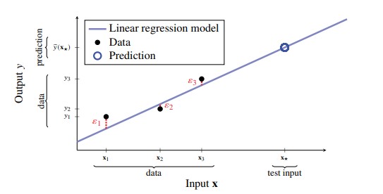Figure 1 - Linear Regression with p=1. Black dots represent data-points, blue line represents learned regression model. Model doesn’t fit data perfectly, so remaining error corresponding to random noise ε for each data-point is shown in red. The model can be used to predict (blue circle) the output ŷ=𝐱★ for a test input 𝐱★

• Since we assume that noise term $\varepsilon$ is random with zero-mean and independent of all variables, it makes sense to set $\varepsilon=0$ for prediction.
• A prediction from a linear regression model is of the general form:

$$\hat{y}(\bf{x_\star})=\hat{\theta}_0 + \hat{\theta}_1 x_{\star 1} + \hat{\theta}_2 \bf{x}_{\star 2} + \cdots + \hat{\theta}_p x_{\star p} = \hat{\bf{\theta}}^{\ T} \bf{x_\star} \tag{3.4}$$

Training a Linear Regression Model

• Want to learn $\bf{\theta}$ from training data $\mathcal{T}=\{\bf{x}\_i, y\_i\}_{i=1}^{n}$ with $n$ data-points with inputs $\bf{x}_i$ and output $y_i$ in the $n\times (p + 1)$ matrix $\bf{X}$ and $n$-dimensional vector $\bf{y}$.

$${\bf{X}}=[\bf{x}_1^T\ \ \bf{x}_2^T\ \ \cdots \ \ \bf{x}_n^T], {\bf{y}}=[y_1\ \ y_2\ \ \cdots \ \ y_n]^T\tag{3.5}$$

• Where each ${\bf{x}}_ i=[1\ \ x_ {i1} \ \ x_ {i2}\ \ \cdots \ \ x_ {ip}]^T$

Defining a Loss Function

• We introduce a loss function, as a way to measure how similar or well our model fits the training data, denoted $L(\hat{y}, y)$ which measures how close the model’s prediction $\hat{y}$ matches the observed data $y$.

• If the model fits the data well ($\hat{y}\approx y$), then the loss function should be small, and vice versa.

• Also define the cost function as the average loss over the training data.

• Training a model amounts to finding the parameter values that minimise the cost:

$$\hat\theta = \arg\min_\theta \frac{1}{n} \sum_{i=1}^n L(\hat{y}(\bf{x}_i; \theta), y_i)\tag{3.9}$$

• Where:
  • $L(\hat{y}(\bf{x}_i; \theta), y_i)$ is the loss function
  • $\sum_{i=1}^n L(\hat{y}(\bf{x}_i; \theta), y_i)$ is the cost function.
• Note that each term in the expression above corresponds to evaluating the loss function for the prediction $\hat{y}(\bf{x}_i; \theta)$
• $\arg\min_\theta$ effectively means “the value of $\bf\theta$ for which the cost function is the smallest”

Least Squares and the Normal Equations

• For regression, a commonly used loss function is the squared error loss:

$$L(\hat{y}(\bf{x}; {\bf{\theta}}), y)=(\hat{y}({\bf{x};{\bf{\theta}}})-y)^2 \tag{3.10}$$

• This loss function is 0 if $\hat{y}({\bf{x}};{\bf{\theta}})=y$ and grows quadratically a the difference between $y$ and the prediction increases.
• The corresponding cost function for the linear regression model, shown in Eq 3.7 can be written using matrix notation as:

$$\begin{align*}J(\theta)&=\frac{1}{n} \sum_{i=1}^{n} (\hat{y}({\bf{x}}_i ; \theta) - y_i)^2 \\ &= \frac{1}{n} ||\hat{\bf{y}} - {\bf{y}} ||_2^2 \\ &= \frac{1}{n} ||{\bf{X}}\theta-{\bf{y}}||_2^2\\ &= \frac{1}{n} ||\epsilon||_2^2\end{align*}\tag{3.11}$$

• Where $||\cdot||_2$ denotes Euclidean vector norm, and $||\cdot||_2^2$ denotes its square.
• This function is known as the least squares cost
• When using the squared error loss for learning a linear regression model from $\mathcal{T}$, we need to solve (Eq 3.12)

&nbsp

$$\begin{align*}\hat{\theta} &= \arg\min_{\theta} \frac{1}{n} \sum_{i=1}^n (\theta^T {\bf{x}}_i - y_i)^2 \\ &=\arg\min_\theta \frac{1}{n} || {\bf{X}}\theta-{\bf{y}}||_2^2 \tag{3.12}\end{align*}$$

• We can denote this using Linear Algebra, in which we want to find the closest vector to $\bf{y}$ in a Euclidean sense in the subspace $\mathbb{R}^n$ spanned by the columns of $\bf{X}$.

$${\bf{X}}^T {\bf{X}}\hat{\theta} = {\bf{X}}^T {\bf{y}}\tag{3.13}$$

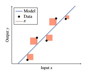Figure 2 - Graphical Representation of Squared Error Loss Function.

• Goal is to choose the model (blue line) such that the sum of squares (denoted in light red) of each error $\varepsilon$
• Equation 3.13 is often referred to as the normal equation and gives the solution to the least squares problem (eq 3.12).
• If ${\bf{X}}^T\bf{X}$ is invertible (which is often the case), then $\hat{\bf{\theta}}$ has the closed form expression:

$$\hat{\bf{\theta}} = ({\bf{X}}^T{\bf{X}})^{-1} {\bf{X}}^T y \tag{3.14}$$

• The fact that this closed-form solution exists is important and is probably the reason for why linear regression + squared error loss is so common in practice.
• Other loss functions lead to optimisation problems that often lack closed-form solutions.

Goal Learn linear regression using squared error loss.

Data Training data $\mathcal{T} = \lbrace {\bf{x}_i , y_ i}\rbrace_{i=1}^{n}$Result Learned parameter vector, $\theta$

1. Construct the matrix $\bf{X}$ and vector $\bf{y}$ according to Eq 3.5
2. Compute $\hat{\bf{\theta}}$ by solving Eq 3.13

Goal Predict with linear regression Data Learned parameter vector $\bf{\theta}$ and test input $\bf{x_\star}$Result Prediction $\hat{y}{\bf{x_\star}}$

1. Compute $\hat{y}({\bf{x_ \star}}) = \hat{\bf{\theta}}^T \bf{x_ \star}$

Maximum Likelihood Perspective (Derivation of Least-Squares)

• We can get another perspective on the least squares method as a maximum likelihood solution
• In this context, the word likelihood refers to the statistical concept of the likelihood function
  • Maximising the likelihood function amounts to finding the value of $\theta$ that makes observing $y$ as likely as possible.
• That is, instead of arbitrarily selecting a loss function, we start with the problem:

$$\hat{\theta} = \arg \max_\theta p({\bf{y}} | {\bf{X}} ; \theta)\tag{3.15}$$

• Here $p({\bf{y}} | {\bf{X}}; \theta)$ is the probability density of all observed outputs $\bf{y}$ in the training data, given all inputs $\bf{X}$ and parameters $\theta$.

• In defining what “likely” means mathematically, we consider the noise term $\varepsilon$ as a stochastic variable with certain distribution

• A common assumption is that the noise terms are independent, each with a Gaussian (normal) distribution with mean zero and variance $\sigma_\varepsilon^2$

$$\varepsilon ~ \mathcal{N}(0, \sigma_\varepsilon^2) \tag{3.16}$$

Stochastic Having a random probability distribution or pattern that may be analysed statistically but may not be predicted precisely.

• This implies that the $n$ observed data points are independent, and $p({\bf{y}} | {\bf{X}} ; \theta)$ factorises as:

$$p({\bf{y}} | {\bf{X}};\theta)=\prod_{i=1}^n p(y_1 | {\bf{x}}_i, \theta)\tag{3.17}$$

• Consider the linear regression model from (3.3), $y=\theta^T {\bf{x}} + \varepsilon$ together with the gaussian noise assumption (3.16) yields the following:

$$\begin{align*} p(y_i | {\bf{x}}_i, \theta)&=\mathcal{N}(y_i;\theta^T {\bf{x}}_i, \sigma_\varepsilon^2)\\ &=\frac{1}{\sqrt{2\pi\sigma_\varepsilon^2}} \exp({-\frac{1}{2\sigma_\varepsilon^2} (\theta^T {\bf{x}_i} - y_i)^2}) \end{align*}\tag{3.18}$$

• Recall that we want to maximise the likelihood with respect to $\theta$. For numerical reasons, it is usually better to work with the logarithm of $p({\bf{y}} | {\bf{X}}; \theta)$.

$$\ln p ({\bf{y}} | {\bf{X}} ; \theta) = \sum_{i=1}^n \ln p (y_i | {\bf{x}}_i, \theta) \tag{3.19}$$

• Since the algorithm is a monotonically increasing function, maximising the log-likelihood (Equation 3.19) is equivalent to maximising the likelihood together. Combining Eq 3.18 and 3.19 yields:

\ln p({\bf{y}} | {\bf{X}} ; \theta) = -\frac{n}{2}\ln(2\pi\sigma_\varepsilon^2) \sigma{i=1}^n (\theta^T {\bf{x}}_i-y_i)^2 \tag{3.20}

• Removing the terms and factors independent of $\theta$ does not change the maximising argument. We can we-write 3.15 as:

\color{gray}\hat{\theta} = \arg \max_\theta p({\bf{y}} | {\bf{X}} ; \theta)\tag{3.15}

\begin{align*}
\hat{\theta} 
&=\arg\max_\theta -\sum_{i=1}^n(\theta^T {\bf{x}}_i-y_i)^2\\
&=\arg\min_\theta\frac{1}{n} \sum_{i=1}^n (\theta^T {\bf{x}}_i - y_i)^2\tag{3.21}
\end{align*}

• We have just derived the equation for linear regression with the last-squares cost (the cost function implied by the squared error loss function, Equation 3.10).
• Hence, using the squared error loss is equivalent to assuming a Gaussian (normal) noise distribution in the maximum likelihood formulation
• Other assumptions on $\varepsilon$ lead to other loss functions.

Categorical Input Variables

• The regression problem is characterised by a numerical output $y$ and inputs of $\bf{x}$ of arbitrary type
• We can handle categorical inputs by first assuming that we have an input variable that takes two different values.
• We refer to these two values as $\text{A}$ and $\text{B}$ respectively, and then create a dummy variable $x$ as:

x=\begin{cases}
0&\text{if A}\\
1&\text{if B}\\
\end{cases}\tag{3.22}

• We use this variable in any supervised machine learning method as if it was numerical.
• For Linear Regression, this effectively gives is a model which looks like:

y=\theta_0 + \theta_1x + \varepsilon=
\begin{cases}
\theta_0+\varepsilon&\text{if A}\\
\theta_0 + \theta_1 + \varepsilon&\text{if B}\\
\end{cases}\tag{3.23}

• The model is thus able to learn and predict two different values depending on whether the input is $A$ or $B$.
• If the categorical variable takes more than two values, say $\{\text{A, B, C, D}\}$ we can make a so-called one-hot encoding by constructing a four-dimensional vector:

{\bf{x}} 
  = \begin{bmatrix}
    x_A & x_B & x_C & x_D
    \end{bmatrix}^T
\tag{3.24}

• In which $x_A=1$ if $\text{A}$ and $x_B=1$ if $\text{B}$ and so on
  • Only one element if $\bf{x}$ will be 1, with the rest being 0
  • This can be used for any type of supervised machine learning methods, not just linear regression

Classification and Logistic Regression

• Can modify the linear regression model to apply it to the classification
• Comes at the cost of not being able to use convenient normal equations, and have to resort to numerical optimisation / iterative learning algorithms

Statistical View of Classification

• Supervised Machine Learning amounts to predicting the output from the input
• Classification amounts to predicting conditional class probabilities, as in Eq 3.25

p ( y = m | {\bf{x}})\tag{3.25}

• $p(y=m|{\bf{x}})$ describes the probability for class m given that we know the input $\bf{x}$.
• The notation $p(y|{\bf{x}})$ implies that we think about the class label $y$ as a random variable.
• Because we choose to model the real world, where data originates as involving a certain amount of randomness (much like the random error $\varepsilon$ in regression).

Example - Voting Behaviour using Probabilities

• Want to construct a model that can predict voting preferences for different population groups.
• Have to face the fact that not everyone in a certain population group will vote for the same political party.
• Can therefore think of $y$ as a random variable which follows a certain probability distribution
• If we know that the vote count in the group of 45 year old women $\bf{x}$ is 13% of the cerise party, 39% for the turquoise party and 48% for the purple party, we could describe it as:

\begin{align*}
  p(y=\text{cerise party} | {\bf{x}}=\text{46 year old women}) = 0.13\\
  p(y=\text{turquoise party} | {\bf{x}}=\text{46 year old women}) = 0.39\\
  p(y=\text{purple party} | {\bf{x}}=\text{46 year old women}) = 0.48
\end{align*}

• In this way the probabilities $p(y|\bf{x})$ describes the non-trivial fact that:
  1. All 45 year old women do not vote for the same party,
  2. The choice of party does not appear to be completely random among 45 year old women either - the purple party is the most popular, and the cerise party ist he least popular.
• This, it is useful to have a classifier which predicts not only a class $\hat{y}$ but a distribution over classes $p(y | {\bf{x}})$

• From the above example, we see the utility of predicting a probability distribution instead of just a single class.
• For binary classification problems ($M=2$) where $y\in\{-1, 1\}$ we train a model $g({\bf{x}})$ for which:

p(y=1 | {\bf{x}}) \text{ is modelled by } g({\bf{x}}) \tag{3.26a}

• By the laws of probabilities, it holds that $p(y=1| {\bf{x}}) + p(y=-1 | {\bf{x}}) = 1$ which means that

p(y=-1|{\bf{x}})\text{ is modelled by } 1-g({\bf{x}}) \tag{3.26b}

• Since $g({\bf{x}})$ is modelled for a probability, it is natural to require that $0\le g({\bf{x}}) \le 1$ for any $\bf{x}$.
• For the multi-class problem, we instead let the classifier return a vector-valued function $\bf{g(x)}$ where:

$$\begin{bmatrix} p(y=1|{\bf{x}})\\ p(y=2|{\bf{x}})\\ \vdots\\ p(y=M|{\bf{x}})\\ \end{bmatrix} \text{ is modelled by } \begin{bmatrix} g_1({\bf{x}})\\ g_2({\bf{x}})\\ \vdots\\ g_M({\bf{x}}) \end{bmatrix} =\bf{g(x)}\tag{3.27}$$

• Each element $g_m({\bf{x}})$ of $\bf{g(x)}$ corresponds to the conditional class probability $p(y=m|{\bf{x}})$.
• Since $\bf{g(x)}$ models a probability vector, we require that each element $g_m(\bf{x}) \ge 0$ and $||\bf{g(x)}||_1 =\sum_{m=1}^M |g_m(\bf{x})|=1$ for any $\bf{x}$.

Logistic Regression Model for Binary Classification

• Logistic Regression is a modification of the linear regression model so that it fits the classification problem.
• Begin with the case for binary classification, in which we wish to learn a function $g({\bf{x}})$ that approximates the conditional probability of the positive class.
• We begin with the linear regression model, which is given by the following equation (with noise term removed):

$$z = \theta_0 + \theta_1 x_1 + \theta_2 x_2 + \cdots + \theta_p x_p =\theta^T \bf{x}\tag{3.28}$$

• This is a mapping that takes $\bf{x}$ as input, and returns $z$, which in this context is called the logit
• Note that $z\in\mathbb{R}$, whereas we need a function which instead returns a value in the interval $[0,1]$.
• The key idea is to use linear regression, and to squeeze $z$ from Eq 3.28 to the interval $[0,1]$ using the logistic function $h(z)=\frac{e^z}{1+e^z}$ which is plotted in the figure below.

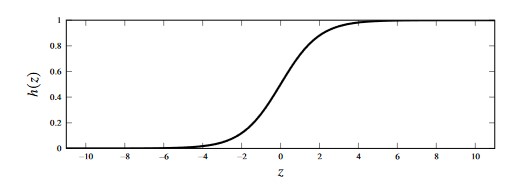
Figure 3  - Plot of the logistic function, given by h(z)=(e^z)/(1+e^z)$

• Substituting the logistic function into our equation for $z$ gives:

$$g({\bf{x}}) = \frac{e^{\theta^T {\bf{x}}}}{1 + e^{\theta^T {\bf{x}}}}\tag{3.29a}$$

• Equation 3.29a is restricted to $[0,1]$ and hence can be interpreted as a probability.
• The function 3.29a is the logistic regression model for $p(y=1|{\bf{x}})$.
• Note that this equation also implicitly gives a model for $p(y=-1 | {\bf{x}})$.

$$p(y=-1 | {\bf{x}}) = 1 - g({\bf{x}}) = 1 - \frac{e^{\theta^T {\bf{x}}}}{1 + e^{\theta^T {\bf{x}}}} = \frac{1}{1+e^{\theta^T {\bf{x}}}} = \frac{e^{-\theta^T {\bf{x}}}}{1 + e^{-\theta^T {\bf{x}}}} \tag{3.29b}$$

• Fundamentally, the logistic regression model is the linear regression model with the logistic scaling function to scale the output at the end.
• Since logistic regression is a model for classification, we omit the loss term $\varepsilon$.
• The randomness in the classification data is modelled by the class probability class construction $p(y=m | {\bf{x}})$ instead of additive noise $\varepsilon$

Training Logistic Regression Model by Maximum Likelihood

• Whilst the addition of the logistic function allows us to use linear regression for binary classification, it means that we cannot use the normal equations for learning $\theta$ due to the non-linearity of the logistic function
• Therefore, to train the model, we learn from the training data $\mathcal{T}=\lbrace {\bf{x}}_i,y_i\rbrace_{i=1}^n$ using the maximum likelihood approach
• Using this Maximum Likelihood approach, learning a classifier amounts to solving the following equation:

$$\hat{\theta}=\arg\max_\theta p({\bf{y}} | {\bf{X}} ; \theta) = \arg\max_\theta \sum_{i=1}^n \ln p(y_i | {\bf{x}}_i; \theta)\tag{3.30}$$

• Equation 3.30 is similar to the training solution for linear regression, in which we assume that all training data-points are independent, and we consider the logarithm of the likelihood function for numerical reasons
• Added $\theta$ explicitly to the notation to emphasise dependence on model parameters.
• Our model of $p(y=1|{\bf{x}};\theta)$ is $g({\bf{x}};\theta)$, which means that we can re-write the log-likelihood component as follows:

$$\ln p(y_i|{\bf{x}_i};\theta)= \begin{cases} \ln g({\bf{x}}_i;\theta)&\text{if }y_i=1\\ \ln(1-g({\bf{x}}_i;\theta))&\text{if }y_i=-1 \end{cases}\tag{3.31}$$

• We can turn the maximisation problem into a minimisation problem by using the negative log-likelihood as a cost function.  

$$\begin{align*} J(\theta) &=-\frac{1}{n}\sum\ln p(y_i|{\bf{x}}_i;\theta)\\ &=\frac{1}{n}\sum_{i=1}{n} \underbrace{ \begin{cases} -\ln g({\bf{x}}_i;\theta)&\text{if }y_i=1\\ -\ln (1-g({\bf{x}}_i;\theta))&\text{if }y_i=-1\\ \end{cases}}_{\text{Binary cross-entropy loss }\mathcal{L}(g({\bf{x}_i;\theta}),y_i)} \end{align*}\tag{3.32}$$

• Note here that the loss that we have derived is the cross-entropy loss.
• For the logistic regression model, we can re-write the cost function given in (Eq 3.32) in greater detail.
  • We consider the case where the binary classes are labelled as $\lbrace-1,1\rbrace$.
• For $y_i=1$, we write:

$$g({\bf{x}}_i;\theta) =\frac {e^{\theta^T{\bf{x}_i}}} {1+e^{\theta^T{\bf{x}_i}}} =\frac {e^{y_i \theta^T {\bf{x}_i}}} {1+e^{y_i \theta^T {\bf{x}_i}}} \tag{3.33a}$$

• And similarly for $y_i=-1$, we write:

$$g({\bf{x}}_i;\theta) =\frac {e^{-\theta^T{\bf{x}_i}}} {1+e^{-\theta^T{\bf{x}_i}}} =\frac {e^{y_i \theta^T {\bf{x}_i}}} {1+e^{y_i \theta^T {\bf{x}_i}}} \tag{3.33b}$$

• Observe how in both cases we get the same expression
• Therefore, we can write (Eq 3.32) compactly as:

$$\begin{align*} J(\theta)&=\frac{1}{N} \sum_{i=1}^{n}-\ln\frac{e^{y_i \theta^T {\bf{x}_i}}}{1+e^{y_i \theta^T {\bf{x}_i}}} =\frac{1}{n}\sum_{i=1}{n}-\ln \frac{1}{1 + e^{-y_i \theta^T {\bf{x_i}}}}\\ &=\frac{1}{n}\sum_{i=1}{n} \underbrace{\ln (1 + e^{-y_i \theta^T {\bf{x_i}}})} _{\text{Logistic loss } \mathcal{L}({\bf{x_i}}, y_i, \theta)} \end{align*} \tag{3.34}$$

• The loss function $\mathcal{L}({\bf{x}}, y_i, \theta)$ shown above (which is a special case of cross-entropy loss) is called the logistic loss (or binomial deviance).
• Learning a logistic regression model then results to solving the following equation to find the optimal $\hat\theta$

$$\hat\theta=\arg\min_\theta\frac{1}{n}\sum_{i=1}{n}\ln(1+e^{-y_i \theta^T {\bf{x_i}}})\tag{3.35}$$

• Unlike linear regression, logistic regression has no closed-form solution so must result to numerical optimisation instead.

Logistic Regression Predictions and Decision Boundaries

Thus far have developed a method for predicting the probabilities for each class for some test input $\bf{x}_\star$.

• Sometimes we just want the best class prediction the model can make without consideration for the class probabilities.
• This is achieved by adding a final step to the logistic regression model which converts the predicted probabilities into class prediction
  • The most common approach is to let $\hat{y}({\bf{x}_\star})$ be the most probable class
  • For the binary classification problem, this can be expressed as shown below.
  • Note that the decision at $g({\bf{x}})=0.5$ is arbitrary.

$$\hat{y}({\bf{x}_\star})= \begin{cases} 1 & \text{if } g({\bf{x}})>r\\ -1 & \text{if }g({\bf{x}})\le r \end{cases}\tag{3.36}$$

Logistic Regression Pseudocode

Learn binary logistic regression

Data: Training data $\mathcal{T}=\lbrace{\bf{x}}_i, y_i\rbrace_{i=1}^{n}$ with output classes $y=\lbrace-1,1\rbrace$

Result Learned parameter vector $\hat\theta$

1. Compute $\hat{\theta}$ by solving (Eq 3.35) numerically

Predict with binary logistic regression

Data Learned parameter vector $\hat\theta$ and test input $\bf{x}_\star$

Result Prediction $\hat{y}({\bf{x}_\star})$

1. Compute $g({\bf{x}_\star})$ using (Eq. 3.29)
2. If $g({\bf{x}_\star})>0.5$ then return $\hat{y}({\bf{x}_\star})=1$ else return $\hat{y}({\bf{x}_\star})=-1$

• In the general case, the decision threshold $r=0.5$ is appropriate.
  • However, in some applications it can be beneficial to explore different thresholds
  • $r=0.5$ minimises the misclassification rate, however, it is not always the most important aspect of a classifier
• For example, it can be more important to mistake a healthy patient as sick (false positive) instead of predict a sick patient as healthy (false negative).
• The addition of class prediction probabilities essentially allows the models to have an “I don’t know” option

Logistic Regression with Multiple Classes

• We can generalise logistic regression to the multi-class problem, where $M>2$.

• One approach is to use the softmax function

• For the binary classification problem we designed a model which return a single scalar value representing $p(y=1|{\bf{x}})$.

• For the multi-class problem, we have to instead return a vector-valued function whose elements are non-negative and sum to 1.

  • We initially use $M$ instances of (Eq 3.28, equation for simple linear regression) and denote each instance $z_m$, with its own set of parameters $\theta_m, z_m=\theta^T_m{\bf{x}}$.
  • We stack all instances of $z_m$ into a vector of logits ${\bf{z}}=\begin{bmatrix}z_1&z_2&\cdots&z_M\end{bmatrix}^T$ and use the soft-max function to replace the logistic function
  • Essentially, use soft-max on the vector of logits instead of the logistic function on each model.

$$\text{softmax}({\bf{z}})\overset{\Delta}{=} \frac{1}{\sum_{m=1}^{M} e^{z_m}} \begin{bmatrix} e^{z_1} & e^{z_2} & \cdots e^{z_M} \end{bmatrix}^T \tag{3.41}$$

• The softmax function takes in a $M$-dimensional vector, and returns a vector with same dimensionality.
  • The output vector from the softmax function always sums to 1, and each element is $\ge 0$.
• We use the softmax function to model the class probabilities (similar to the use of the logistic function in the binary classification case).

$${\bf{g}}({\bf{x}})=\text{softmax}({\bf{z}}), \ \ \ \ \ \ \ \ \ \ \ \ \ \text{where }\bf{z}= \begin{bmatrix} \theta_1^T{\bf{x}}\\ \theta_2^T{\bf{x}}\\ \vdots\\ \theta_M^T{\bf{x}}\\ \end{bmatrix} \tag{3.42}$$

• We can also write out the individual class probabilities (i.e., elements of vector $\bf{g(x)}$) as:

$$g_m({\bf{x}})=\frac{e^{\theta^T_m {\bf{x}}}}{\sum_{j=1}{M} e^{\theta^T_j {\bf{x}}}}, \ \ \ \ \ \ \ \ \ \ \ \ \ \ \ \ \forall m=1, \cdots, M \tag{3.43}$$

• Note that this construction uses $M$ parameter vectors $\theta_1, \cdots, \theta_M$, which means that the number of parameters that need to be learned grows as $M$ increases.

Training Logistic Regression with Multiple Classes

• As with the binary logistic regression model, we can use the concept of maximum likelihood to train our model.
• For this, we will use $\theta$ to denote all model parameters, $\theta=\lbrace\theta_1,\cdots,\theta_M\rbrace$.
• Since $g_m({\bf{x}}_i; \theta)$ is our model for $p(y_i=m|{\bf{x}}_i)$, the cost function for the cross-entropy loss for the multi-class problem is given as:

$$J(\theta)=\frac{1}{n}]\sum_{i=i}^{n} \underbrace{-\ln g_{y_i} ({\bf{x}}_i;\theta)}_{\text{Multi-class cross-entropy loss}}\tag{3.44}$$

• Note that this multi-class cross-entropy loss is denoted $\mathcal{L}({\bf{g}}({\bf{x}}_i;\theta),y_i)$
• We can insert the model we developed in (Eq 3.43) into the loss function (Eq 3.44) to give the cost function to optimise for the multi-class logistic regression problem.

$$J(\theta)=\frac{1}{n}\sum_{i=1}^{n}(-\theta_{y_i}^T {\bf{x}}_i + \ln \sum_{j=1}^{M} e^{\theta_j^T{\bf{x}}_i})\tag{3.45}$$

Polynomial Regression and Regularisation

• Linear and Logistic Regression may appear rigid and non-flexible compared to $k$-NNs and Decision Trees as they are comprised of purely straight lines

• However, both models are able to adapt to the training data well if the input dimension $p$ is large relative to the number of data points $n$.

• We can increase the input dimension by performing a non-linear transformation of the input.

• A simple way of doing this is to replace a one-dimensional input $x$ with itself raised to different powers (which turns this into polynomial regression)

  • The same can be done for the logit in logistic regression.

$$y=\theta_0 + \theta_1x + \theta_2x^2 + \theta_3 x^3 + \cdots + \varepsilon \tag{3.46}$$

• Consider that in the original linear regression model, if we let $x_1=x, x_2=x^2, x_3=x^3$, this is still a linear model, with input ${\bf{x}}=\begin{bmatrix}1&x&x^2&x^3\end{bmatrix}$

  • However, in doing this, the input dimensionality has increased from $p=1$ to $p=3$.

• Non-linear input transformations can be very useful, but it effectively increases $p$ and can easily over fit the model to noise.

• In the car stopping example, we have our original data, and add a $1$ for the offset, term, and $x^2$ for the second order term to produce a new matrix

$$\begin{align*} X=\begin{bmatrix} 1 & 4.0 & 16.0 \\ 1 & 4.9 & 24.0 \\ 1 & 5.0 & 25.0 \\ \vdots & \vdots & \vdots \\ 1 & 39.6 & 1568.2 \\ 1 & 39.7 & 1576.1 \\ \end{bmatrix}, \ \ \ \ \ \ \ \ \ \ \ \theta = \begin{bmatrix}\theta_0\\\theta_1\\\theta_2\end{bmatrix}, \ \ \ \ \ \ \ \ \ \ \ \ y = \begin{bmatrix} 4.0 \\ 8.0 \\ 8.0 \\ \vdots \\ 134.0 \\ 110.0 \end{bmatrix} \end{align*} \tag{3.47}$$

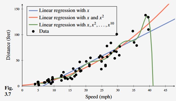
Figure 4 - 

  Learning the car stopping distance with linear regression, second-order polynomial regression and 10th order polynomial regression. From this, we can see that the 10th degree polynomial is over fitting to outliers in the data making it less useful than even ordinary linear regression (blue).

Regularisation

• One way to avoid the over-fitting of the model is to carefully select which inputs (transformations) to include.

  • Forward Selection Strategy Add one input at a time
  • Backward Elimination Strategy Remove inputs that are considered to be redundant

• We can additionally evaluate different candidate models, and compare using cross validation (discussed in Chapter 4.)

• Additionally, we can perform regularisation, which is the idea of keeping the parameters $\hat\theta$ small unless the data really convinces us otherwise.

• There are different ways to implement this mathematically, which result in different regularisation techniques.

L2 Regularisation

• To keep $\hat\theta$ small, an extra penalty term $\lambda ||\theta ||_2^2$ is added to the cost function when using L^2 regularisation

• Here, $\lambda\ge0$ is referred to as the regularisation parameter (a hyperparameter chosen by the user, which controls the strength of regularisation effect).

  • This penalty term prevents over fitting
  • Original cost function only rewards fit to training data, the regularisation term prevents overly large parameter values at the cost of a slightly worse fit
  • Therefore, important to choose the value of the regularisation parameter $\lambda$ wisely.
  • $\lambda=0$ has no regularisation effect whilst $\lambda\rightarrow\infty$ will force all parameters $\hat\theta$ to 0.

• Adding $L^2$ regularisation to the linear regression model with squared loss error (Eq 3.12) yields the following equation

$$\hat\theta=\arg\min_\theta\frac{1}{n} || {\bf{X}}\theta-y||_2^2 + \lambda ||\theta||_2^2 \tag{3.48}$$

• Just like the non-regularised problem, Eq 3.48 has a closed-form solution given by a modified version of the normal equations:

$$\def\x{{\bf{X}}} (\x^T \x _ n\lambda {\bf{I}}_{p+1})\hat\theta=\x^T y\tag{3.49}$$

• Note that in this equation ${\bf{X}}_{p+1}$ is the identity matrix of size $(p+1)\times(p+1)$.

• This particular application of regularisation is referred to as ridge regularisation.

• The concept of regularisation is not limited to linear regression

  • The same $L^2$ penalty can be applied to any method that involves the optimisation of a cost function

• For example, here is the $L^2$ regularisation applied to logistic regression

$$\hat\theta=\arg\min_\theta\frac{1}{n}\sum_{i=1}^{n} \ln (1 + \exp(-y_i \theta^T {\bf{x}}_i)) + \lambda || \theta||_2^2\tag{3.50}$$

• Logistic regression is commonly trained using Eq. 3.50 instead of Eq 3.29.
  • This reduces possible issues with over fitting
  • Additionally, have issues with model diverging with some datasets unless $L^2$ is used.

Generalised Linear Models

This section has been omitted as it is not part of the assessable content for this course