Lindholm et al, Chapter 4

A summary of Lindholm Chapter 4 - Understanding, Evaluating and Improving Performance

• At present, have just trained models, and assumed that they are performant
• This section discusses how to evaluate and improve the performance of models in production

Expected New Data Error E_new: Performance in Production

This section is really also regarding model selection

• Define new error function $E(\hat{y},y)$ which encodes purpose of classification and regression
  • Compares prediction $\hat{y}({\bf{x}})$ to measured data point $y$.
  • Returns a small value if $hat{y}$ is a good prediction, and a larger value otherwise
• Can consider different error functions, depending on what properties of prediction are most important.
• Our default choices are as follows:
  • Average misclassification (calculated as misclassification rate = 1 - accuracy)

$$\text{Misclassification}:\ E(\hat{y}, {y})\triangleq \mathbb{I}(\hat{y}\ne y) \begin{cases} 0&\text{if } \hat{y}=y\\1&\text{if }\hat{y}\ne y\end{cases}\tag{4.1a}\\$$

• Squared Error for regression problems. This is similar to the loss function $L(\hat{y},y)$.
  • Loss function is used when learning/training
  • Error function is used to analyse performance of a model that has already been trained

$$\text{Squared Error}:\ E(\hat{y}, y)\triangleq \mathbb{I} (\hat{y}-y)^2 \tag{4.1b}$$

Supervised Learning as Inputs over Random Distribution

• In the end, supervised learning amounts to designing a method that performs well on new, unseen data.

• The performance can be mathematically understood as the average of error function (how often classifier is right)

• To mathematically model this data, introduce distribution over data, denoted $p({\bf{x}}, y)$.

  • Now consider $\bf{x}$ as a random variable with a probability distribution

• Regardless o the classification or regression method chosen, it learns from training data $\mathcal{T}=\{{\bf{x}}_i, y_i\}_{i=1}^{n}$ and return predictions $\hat{y}({\bf{x}_\star})$ for any new input $\bf{x_\star}$.

• Now denote the prediction as $\hat{y}({\bf{x}};\mathcal{T})$ tp emphasise that the model depends on the training data $\mathcal{T}$.

Integration-Based Error Rate

• Previous,y discussed how model predicts output for one or a few test inputs $\bf{x_\star}$.
• Now consider averaging the error function over all data points with respect to the distribution $p({\bf{x}}, y)$
  • Refer to this as the expected new data error

$$E_{\text{new}} \overset{\Delta}{=} \mathbb{E}_\star [ E ( \hat{y}({\bf{x_\star}}; \mathbb{T}), y_\star)]\tag{4.2}$$

• In this equation $\mathbb{E}_\star$ is the expectation over all possible test data points with respect to the distribution $({\mathbb{x_\star}}, y_\star)~p({\bf{x}},y)$

$$\mathbb{E}_\star [ E ( \hat{y}({\bf{x_\star}}; \mathbb{T}), y_\star)]=\int E(\hat{y}({\bf{x_\star}};\mathcal{T}), y_\star) p({\bf{x_\star}},y_\star) d{\bf{x_\star}} dy_\star \tag{4.3}$$

• The model, regardless of its type is trained on a given training dataset $\mathcal{T}$.

• In Eq 4.2, we average over all possible test data points $({\bf{x_\star}}, y_\star)$.

• Thus, $E_\text{new}$ describes how well the model generalises from the training data $\mathcal{T}$ to new situations

• We can extend this concept to the computation of the training error:

$$E_\text{train} \overset{\Delta}{=} = \frac{1}{n}\sum_{i=1}^n E(\hat{y}({\bf{x}}_i;\mathcal{T}), y_i)\tag{4.4}$$

• Note that $\{{\bf{x}}_i, y_i\}_{i=1}^{n}$ is the training data $\mathcal{T}$

• $E_\text{train}$ describes how well a method performs on specific data it was trained on

  • Doesn’t give any insight on how the model performs on new, unseen data

• $E_\text{new}$ describes how well a model performs “in production” on new data.

• A model that fits the training data well (small $E_\text{train}$) might still have large $E_\text{new}$ when faced with new data

  • The best strategy to minimise $E_{new}$ is therefore, not necessarily to minimise $E_\text{train}$.
  • Furthermore, misclassification (Eq 4.1a) is unsuitable as an optimisation objective as it is discontinuous and has a derivative of zero almost everywhere
  • We can choose better loss function such as gradient boosting (Ch 7) and support vector machines (Ch 8)

• Not all models are trained by explicitly training a loss function (e.g. $k$-NN)

• In practice, can never compute $E_\text{new}$ - we do not know true $y$ in practice by definition

• We can instead attempt to estimate $E_\text{new}$.

Estimating E new

• There are several motivations for estimating $E_\text{new}$.
  • Judging if performance is satisfying (whether $E_\text{new}$ is small enough), or whether more work should be put into the solution and/or more training data should be collected
  • Choosing between different methods
  • Choosing hyper-parameters in order to minimise $E_\text{new}$
  • Reporting expected performance to customer.

Cannot Estimate E new from Training Data

• Consider that $\mathcal{T}$ contains samples from $p({\bf{x}}, y)$.
• Training data is assumed to have been collected under similar circumstances to that which the train model is being used.
• When an expected value cannot be computed in closed form (e.g. Eq 4.2), we can approximate the expected value by a sample average
• We can attempt to approximate the integral (expected value) by a finite sum.
• However, the data points used to perform this approximation is data that the model was trained on, and thus we cannot have any guarantee on the performance when evaluated on previously unseen data.

Hold-Out Validation Data

• To circumvent the issue presented before, we can partition the data to create a set of hold-out validation data denoted $\def\rq{'}\lbrace{\bf{x}}_j\rq, y_j\rq \rbrace$ which is not in $\mathcal{T}$ used for training.
• We can then use this data to compute the estimated performance of the model, known as the hold-out validation error

$$\def\rq{``} E_\text{hold-out} \overset{\Delta}{=} \frac{1}{n_v} \sum_{j=1}^{n_v} E(\hat{y}({\bf{x}}_j\rq;\mathcal{T}), y_j\rq)\tag{4.6}$$

• In this way, not all data will be used for training, but some data points will be saved and used for only computing $E_\text{hold-out}$.
• However, you have to be careful when splitting your dataset
  • Someone might have sorted the dataset for you, so you must shuffle the samples in your data before splitting.
• Therefore, assuming that both training and validation (hold-out) data is drawn from the same probability distribution, then we have that:

$$E_\text{hold-out} = E_\text{new}$$

• However, this does not tell us how close $E_\text{hold-out}$ is to $E_\text{new}$ for a single experiment
• The variance of $E_\text{hold-out}$ will decrease if the size of the validation dataset.
  • Thus, for sufficiently large $E_\text{hold-out}$, the above equation holds
• This is not an issue if there is a lot of data.
  • However, if dataset is limited then have a trade-off between wanting to know out $E_\text{hold-out}$ and decreasing our error rate $E_\text{new}$ (more training data = less error)

k-Fold Cross-Validation

• To avoid setting aside validation data but still obtain an estimate of $E_\text{new}$, we could perform a two-step procedure:

  1. Split available data into training and hold-out validation set. Train the model on the training dataset and compute $E_\text{hold-out}$ using the hold-out validation data
  2. Train the model again using entire dataset.

• This is better, but not perfect - to get a small variance in the estimate, must put a lot of data in hold-out validation dataset.

• This means that model trained in step (1) can vary quite significantly to resulting model trained on entire dataset.

• We can build on this idea to derive the k-fold cross-validation method by repeating the hold-out validation procedure multiple times:

  1. Split the dataset into k batches of similar size and let $\ell=1$
  2. Take batch $\ell$ as the hold-out validation data and the remaining batches as training data
  3. Train the model on the training data and compute $E_\text{hold-out}^{(\ell)}$ as average error on hold-out validation data.
  4. If $\ell< k$ set $\ell\leftarrow\ell+1$ and return to (ii). If $\ell=k$ then compute k-fold cross validation error

  $$E_\text{k-fold}\overset{\Delta}{=}\frac{1}{k}\sum_{\ell=1}^{k} E_\text{hold-out}^{(\ell)}$$

  5. Train the model again, using the entire dataset

• Using the k-fold cross-validation method, we get a model which is trained on all the data, as well as an approximation of $E_\text{new}$ denoted $E_\text{k-fold}$.

  • Whilst $E_\text{hold-out} $ was an unbiased estimate of $E_\text{new}$ (at the cost of setting aside hold-out validation data), this is not the case for $E_\text{k-fold}$.
  • However, with large enough $k$, this is a sufficiently good approximation

Why does this work?

• The intermediate models are trained on $\frac{1-k}{k}$ of the data
• If k is sufficiently large, then they are quite similar to the final model since they are trained on almost the same dataset
• Furthermore, each intermediate $E_\text{hold-out}^{(\ell)}$ is an unbiased but high-variance estimate of $E_\text{new}$ for the corresponding $\ell^\text{th}$ intermediate model
• Since all intermediate models and the final model are similar, $E_\text{k-fold}$ is approximately the average of k high-variance estimates of $E_\text{new}$ for the final model
• When averaging estimates, variance decreases and $E_\text{k-fold}$ will become a better estimates of $E_\text{new}$ than the intermediate $E_\text{hold-out}^{(\ell)}$.

Training Time

• Training is typically discussed as a procedure that is executed once
• In k-fold cross-validation, the training is repeated O(k) times
• For methods such as linear regression, the actual training is usually done in milliseconds, so doing it an extra O(k) times might not be a problem in practice
• If the training is computationally demanding (as in Deep Neural Networks) it becomes a rather cumbersome procedure, and $k=10$ might be more practically feasible.
• If there is a lot of data available, it is also an option to use the hold-out approach.

Using a Test Dataset

• In practice, important to choose $E_\text{k-fold}$ or $E_\text{hold-out}$ with hyper-parameters so that the error is minimised
• However, we cannot use $E_\text{train}$ to estimate the new data error $E_\text{new}$ (select models based on $E_\text{train}$)
  • If we do this, we risk over-fitting tot he validation data, resulting in $E_\text{k-fold}$ being overly optimistic estimate of the actual new data error
• If important to have good estimate of the final $E_\text{new}$, set aside another hold-out dataset - this is our test set.
• This test set should only be used once (after selecting models and hyper-parameters) to estimate $E_new$ for the final model.

Augmenting Training Set

• In problems where training data is expensive, common to increase training dataset using more or less artificial techniques.
• Can duplicate data and add noise to duplicated versions, to use simulated data, or use data from different but related problem.
• In this case, training data $\mathcal{T}$ is no longer drawn from $p(\bf{x},y)$.

The Training Error-Generalisation Gap Decomposition of E new

This section discusses over-fitting and under-fitting

• The core goal of supervised machine learning is to design method with small $E_\text{new}$
• Can gain more insights and better understand the behaviour of these methods by further reasoning about $E_\text{new}$
• Introduce training-data averaged $E_\text{new}$ and $E_\text{train}$.

$$\bar{E}_\text{new}\overset{\Delta}{=}\mathbb{E}_{\mathcal{T}}[E_\text{new}(\mathcal{T})]\tag{4.8a}$$

$$\bar{E}_\text{train}\overset{\Delta}{=} \mathbb{E}_{\mathcal{T}}[E_\text{train}(\mathcal{T})]\tag{4.8b}$$

• Here $\mathbb{E}_\mathcal{T}$ denotes the expected value with respect to the training set $\mathcal{T}=\lbrace{\bf{x}}_i, y_i\rbrace_{i=1}^n$
  • This is based on the assumption that the training dataset consists of independent draws from some probability distribution $p({\bf{x}}_i, y_i)_{i=1}^n$
• Know that $E_\text{train}$ cannot be used to estimate $E_\text{new}$, but generally, it holds that:

$$\bar{E}_\text{train} \lt \bar{E}_\text{new}\tag{4.9}$$

• That is, a method performs worse on new, unseen data than on training data
• A method’s ability to perform well on unseen data after being trained is referred to as its ability to generalise from training data
• Therefore, call the difference between $\bar{E}_\text{new}$ and $\bar{E}_\text{train}$ the generalisation gap

$$\text{generalisation gap}\overset{\Delta}{=}\bar{E}_\text{new}-E_\text{train}\tag{4.10}$$

$$\bar{E}_\text{new}=\bar{E}_\text{train}+\text{generalisation gap}\tag{4.11}$$

Generalisation Gap Factors

• Size of generalisation gap depends on method and problem
• The more a method adapts to training data, the larger the generalisation gap

• Framework for how much method adapts to training data is given by Vapnik-Chervonenkis (VC) dimension

• Probabilistic bounds on generalisation gap can be derived, but are typically rather conservative.

• Can use the terms model complexity or model flexibility which refers to the model’s ability to adapt to patterns in the training data

• A model with high complexity (such as fully connected DNN, deep trees or k-NN with small k) can describe complicated input-output relationships

• However, models with low complexity (such as logistic regression) is less flexible in terms of what functions it can describe

• Model complexity for parametric models dependent on number of learnable parameters and regularisation techniques

• This idea of model complexity is an oversimplification but is still useful for intuition

• Typically, higher model complexity implies larger generalisation gap

• $\bar{E}_\text{train}$ decreases as model complexity increases, whereas $\bar{E}_\text{new}$ typically attains a minimum value for some intermediate model complexity value.

  • Model complexities that are too low or too high increase $\bar{E}_\text{new}$.
  • Over-fitting: Model complexity that is too high ($\bar{E}_\text{new}$ is higher than it would be with a less-complex model)
  • Under-fitting: Model complexity that is too low
  • The point at which $\bar{E}_\text{new}$ obtains a minimum value is referred to as a “balanced fit”

  

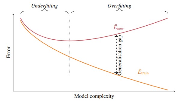
Figure 1 - Over-fitting vs Under-fitting

• In the figure above, we observe the behaviour of $\bar{E}_\text{new}$ and $\bar{E}_\text{train}$ as model complexity increases
  • $\bar{E}_\text{train}$ decreases as the model complexity increases
  • However, $\bar{E}_\text{new}$ does not necessarily decrease as the model complexity increases.
  • We ideally want to choose a model with complexity such that $\bar{E}_\text{new}$ is minimised.

Binary Classification Example

• Consider simulated binary classification input with two dimensional input ${\bf{x}}=\begin{bmatrix}x_1, x_2\end{bmatrix}^T$

• Since problem is simulated, we know that $ p({\bf{x}},y) $ (that $ \bf{x} $ is drawn from some probability distribution)

• In this problem $p(\bf{x})$ is a uniform distribution on the square $[-1,1]^2$ and $p(y|{\bf{x}})$ defined as follows:

  • All points above dotted curve are red with probability 0.8
  • All points below curve are red with probability 0.8.

• The optimal classifier in terms of minimal $E_\text{new}$ would have the dotted line as its decision boundary and achieve $E_\text{new}=0.2$.

  

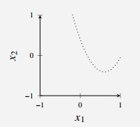
  Figure 2 -   Optimal Decision Boundary for Classification Problem

• We generate a training dataset with $n=200$ samples.

• Using this training data, we train three $k$-NNs with $k=\lbrace70, 20, 2\rbrace$ as shown in the figure below

  

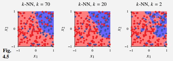
  Figure 3 -   Example of Over-fitting and Under-fitting in KNN Classification

• We see that $k=70$ gives the least flexible model and $k=2$ gives the most flexible model

• We see that in the figure $k=2$ (right) adapts too much to the data

• Conversely $k=70$ (left) is rigid enough to not adapt to the noise, but might be too inflexible to adapt to the true decision boundary

• By creating more testing data, we can compute $E_\text{train}$ and $E_\text{new}$.

  • Since in this example, the data is simulated, we can estimate $E_\text{new}$ numerically by creating more test data and computing it.

• This resembles Figure 1 above, except that $E_\text{new}$ is smaller than $E_\text{train}$ for some values of $k$.

• We observe in the tabulated values that the generalisation gap $\overset{\Delta}{=} \bar{E}_\text{new} - \bar{E}_\text{train}$

• For the values of $k$ shown, we observe that $\bar{E}_\text{new}$ is smallest for $k=20$

  • This suggests that by extension $k=2$ suffers from over-fitting and $k=70$ suffers from under-fitting

• A key factor in the size of the generalisation gap is the size of the training set.

  • In general, the more training data, the smaller the generalisation gap
  • However, $\bar{E}_\text{train}$ typically increases as $n$ increases, since most models are unable to fit all training data-points well if there are too many

  

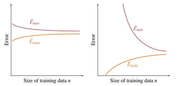
  Figure 4  - Behaviour of Training Models with increase in size of training data. Simple model (left) vs complex model (right)

• More complex model will attain smaller $\bar{E}_\text{new}$ for a large enough $n$.

• The generalisation gap is larger for a more complex model, especially when the training dataset is small.

Reducing E new in Practice

• Overarching goal in supervised learning to reduce $E_\text{new}$

• Eq (4.11) from before defines that $E_\text{new} = E_\text{train} + \text{generalisation gap}$.

• This implies that to reduce $E_\text{new}$ we both need to reduce $E_\text{train}$ and $\text{generalisation gap}$

• The new data error $E_\text{new}$ will, on average, not be smaller than the training data $E_\text{train}$

  • Therefore, if $E_\text{train}$ is much larger than the value of $E_\text{new}$ required, need to re-think the problem and method chosen to solve it

• The generalisation gap and $E_\text{new}$ decrease as $n$ increases.

  • If possible, increasing the size of the training data may significantly decrease $E_\text{new}$

• Making the model more flexible decreases $E_\text{train}$ but often increase the generalisation gap.

  • Making the model less flexible decreases the generalisation gap, but increases $E_\text{train}$

• Therefore, the optimal trade-off (to minimise $E_\text{new}$) is obtained when when neither the generalisation gap nor $E_\text{train}$ is zero.

• We can monitor $E_\text{train}$ and estimate $E_\text{new}$ with cross-validation to obtain the following conclusions:

  • If $E_\text{hold-out} \approx E_\text{train}$ (small generalisation gap, possibly under-fitting), it might be beneficial to increase model flexibility by loosening regularisation, increasing the model order (more parameters to learn), etc.
  • If $E_\text{train}$ is close to zero and $E_\text{hold-out}$ is not (possibly over-fitting), it might be beneficial to decrease the model flexibility by tightening the regularisation, decreasing the order (fewer parameters to learn), etc.

Shortcomings of Model Complexity Scale

• When there is one hyperparameter to choose, it is often easy to determine what to do (as in Figure 1)
• However, when there are multiple hyper-parameters (or competing methods) it is important to realise that one-dimensional complexity as shown before doesn’t properly address the space for all possible choices
• It is possible for a method to have a smaller generalisation gap than another method without having larger training error.
• The one-dimensional complexity can be misleading for intricate deep-learning models
  • Not even sufficient for relatively simple problem of jointly choosing degree of polynomial regression and regularisation parameter

Example - Training Error and Generalisation Gap for Regression

• Consider a simulated problem with $n=10$ generated using $x~\mathcal{U}[-5,10]$, $y=\min(0.1x^2,4)+\varepsilon$ and $\varepsilon~\mathcal{N}(0,1)$

• We consider the following regression methods:

  • Linear Regression with $L^2$ regularisation
  • Linear regression with quadratic polynomial and $L^2$ regularisation
  • Linear regression with third-order polynomial and $L^2$ regularisation
  • Regression tree
  • Random forest with 10 regression trees

• For each of these methods, try a few different values of parameters (regularisation parameters, tree depth) and compute $\bar{E}_\text{train}$ and the generalisation gap

  

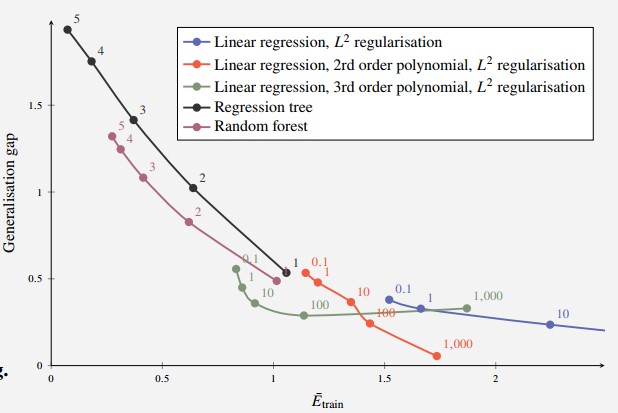
  Figure 5  - Evaluation of training loss and generalisation gap

• For each method, the hyperparameter that minimises $\bar{E}_\text{new}$ is the value that is the closest to the origin since $\bar{E}_\text{new}=\bar{E}_\text{train}+\text{generalisation gap}$

• When comparing different methods, the problem is more complex than that presented before.

• Takeaway: Relationships are intricate, problem-dependent and impossible to describe using the methodology above

  • Observe the second-order polynomial (red) vs the third-order polynomial (green) linear regression
    • For some values of the regularisation parameter, the training error decreases without increasing the generalisation gap
  • Similarly, the generalisation gap is smaller while the training error remains the same (for the random forest than for the tree)

• We can simplify this by introducing the bias-variance decomposition

Bias-Variance Decomposition of E_new

• Introduce another decomposition of $\overline{E}_\text{new}$ using squared bias and variance.

Recap of Bias and Variance

• Consider an experiment with an unknown constant (true value) $z_0$ which we would like to estimate.
• $z$ are our measurements of $z_0$, which are drawn from some random distribution
  • Since $z$ is a random variable, it has some mean which is denoted as $\mathbb{E}[z]\equiv \overline{z}$.
• Now introduce the concepts of bias and variance

$$\text{Bias}: \overline{z}-z_0\tag{4.12a}$$

$$\text{Variance}: \mathbb{E}[(z-\overline{z})^2]=\mathbb{E}[z^2]-\overline{z}^2\tag{4.12b}$$

• Variance: How much the result varies each time it is sampled

• Bias: Systematic, constant error in $z$ that remains regardless of number of times sampled.

• If we consider the squared error between $z$ and $z_0$ to as a metric of how good the estimator $z$ is, wegt can re-write it in terms of the variance and squared bias:

$$\begin{align*} \mathbb{E}[(z-z_0)^2]&=\mathbb{E}[((z-\overline{z}) + (\overline{z}-z_0))^2]=\\ &=\underbrace{\mathbb{E}[(z-\overline{z})^2]}_{\text{Variance}} +2 \underbrace{(\mathbb{E}[z] - \overline{z})}_{\text{0}} (\overline{z}-z_0) + \underbrace{(\overline{z}-z_0)^2}_{\text{bias}^2} \end{align*}\tag{4.13}$$

• The average squared error between $z$ and $z_0$ is the sum of the squared bias and variance.
• To obtain small expected squared error, have to consider both the bias and variance - that is, both values need to be small.

Bias and Variance in a Machine Learning Context

• Consider the regression problem with squared error function (SSE) for the sake of simplicity.

  • This concept and the intuition behind it carries over to classification as well.

• In this context, $z_0$ corresponds to the true relationship between input and output.

• $z$ corresponds to the model learned from the trained data.

  • Since the training data collection includes randomness, the model learned from it will also be random.

• Make the assumption that the true relationship between the input $\bf{x}$ and the output $y$ can be described using (a possibly very complicated) function $f_0({\bf{x}})$ plus some independent noise term $\varepsilon$.  

$$\def\x{{\bf{x}}} y=f_0(\x)+\varepsilon, \text{ with } \mathbb{E}[\varepsilon]=0 \text{ and var}(\varepsilon)=\sigma^2\tag{4.14}$$

• Use the notation $\hat{y}({\bf{x}};\mathcal{T})$ to denote the model trained on some training data $\mathcal{T}$.
  • This is our random variable, which corresponds to $z$ defined above.
• We also introduce the average trained model, which corresponds to $\overline{z}$:

$$\overline{f}({\bf{x}})\overset{\Delta}{=}\mathbb{E}_\mathcal{T}[\hat{y}({\bf{x}};\mathcal{T})]\tag{4.15}$$

• $\mathbb{E}_\mathcal{T}$ denotes the expected value over $n$ training data points drawn from some probability distribution $p({\bf{x}}),y$.

• Therefore, $\overline{f}({\bf{x}})$ is the (hypothetical) average model achieved if the model could be trained an infinite number of times on different training sets of size $n$ and then compute the average of all of those models.

• From before, we have the definition of $\overline{E}_\text{new}$ defined for regression with squared error:

$$\overline{E}_\text{new}=\mathbb{E}_\mathcal{T}[\mathbb{E}_\star[(\hat{y}({\bf{x_\star}};\mathcal{T})-y_\star)^2]]\tag{4.16}$$

• We can alternatively denote Eq 4.16 as

$$\overline{E}_\text{new}=\mathbb{E}_\star[\mathbb{E}_\mathcal{T}[(\hat{y}({\bf{x_\star}};\mathcal{T})-f_0({\bf{x_\star}})-\varepsilon)^2]]\tag{4.17}$$

• Extending 4.13 to also include the zero-mean noise term $\varepsilon$ gives the following expression inside the expected value $\mathbb{E}_\star$ in Eq 4.17 as:

$$\def\e{\mathbb{E}} \def\x{{\mathbb{x}}} \def\t{\mathcal{T}} \def\yhat{\hat{y}} \def\model{\yhat({\bf{x_\star}};\t)} \e_\t[(\underbrace{\model}_\text{``z''} - \underbrace{f_0({\bf{x_\star}})}_{\text{``}z_0\text{''}}-\varepsilon)^2]\\ \ \\$$

• This equation is effectively the application of Eq 4.13 applied to supervised machine learning
  • In $\overline{E}_\text{new}$, we also have the expectation over new data points $\mathbb{E}_\star$.
  • We can incorporate that expected value into the expression to form a new decomposition of $E_\text{new}$.

$$\def\e{\mathbb{E}} \def\x{{\mathbb{x}}} \def\xstar{{\bf{x_\star}}} \def\t{\mathcal{T}} \def\yhat{\hat{y}} \def\model{\yhat({\bf{x_\star}};\t)} \overline{E}_\text{new}= \underbrace{\e_\star[(\overline{f}(\xstar)-f_0(\xstar))^2]} _{\text{Bias}^2} + \underbrace{\e_\star[\e_\t[(\yhat(\xstar;\t)-\overline{f}(\xstar))^2]]} _{\text{variance}} + \underbrace{\ \ \ \ \sigma^2 \ \ \ \ }_ \text{Irreducible error} \tag{4.19}$$

• In this new decomposition, the squared bias term $\def\e{\mathbb{E}}\def\xstar{{\bf{x}_\star}}\e_\star[(\overline{f}(\xstar)-f_0(\xstar))^2]$ describes how much the average trained model $\overline{f}({\bf{x_\star}})$ differs from the true $\overline{f}({\bf{x}})$ averaged over all possible test data points $\bf{x_\star}$.

• The variance term $\def\e{\mathbb{E}}\def\t{\mathcal{T}}\def\yhat{\hat{y}}\def\xstar{{\bf{x}_\star}}\e_\star[\e_\t[(\yhat(\xstar;\t)-\overline{f}(\xstar))^2]]$ describes how much $\hat{y}({\bf{x_\star}};\mathcal{T})$ varies each time the model is trained on a different training set.

• For the bias term to be small, the model must be flexible enough such that $\overline{f}({\bf{x}})$ can be close to $f_0({\bf{x}})$ (at least in regions where $p({\bf{x}}))$ is large).

• If the variance term is small, the model is not very sensitive to exactly which data points happened (or happened not to be) in the training data.

• The irreducible error $\omega^2$ is a byproduct of the assumption in Eq 4.14 in which it is not possible to predict $\varepsilon$ since it is a random error independent of all other variables.

  

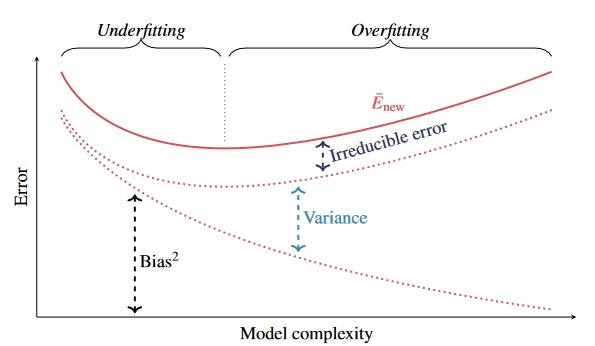
  Figure 6 - Model Complexity vs Error considering the bias-variance decomposition of Enew. Observe that low model complexity means high bias. More complex models adapts to noise in the training data which results in higher variance. This means that to achieve small Enew we need to select a suitable model complexity level. This is called the bias-variance tradeoff.

Factors Affecting Bias and Variance

• We can use Bias and Variance to define model complexity
• A model with high complexity means low bias and high variance.
  • Conversely, low model complexity means high bias and low variance.
• The more flexible the model is, the more it will adapt to the training data (including the actual data points present as well as any noise)
• A less flexible model can be too rigid to capture the true relationship $f_0({\bf{x}})$ between the inputs and outputs - this effect is described by the squared bias term.

Example: Bias-Variance Tradeoff for $L^2$ Regularised Linear Regression

• Consider a simple example in which $p(x,y)$ follows the probability distributions:

$$x~\mathcal{U}[0,1]$$

$$y=5-2x+x^3+\varepsilon, \ \ \ \ \ \varepsilon~\mathcal{N}(0,1)\tag{4.20}$$

• Let the training data consists of only $n=10$ data points.
• Attempt to model the data using linear regression with a 4th order polynomial denoted

$$y=\beta_0+\beta_1x + \beta_2x^2+\beta_3x^3+\beta_4x^4+\varepsilon\tag{4.21}$$

• Since 4.20 is a special case of 4.21, and the squared loss corresponds to gaussian noise, we have a zero-bias model if we train using squared loss error.

• However, learning 5 parameters from only 10 data points leads to very high variance.

  • Therefore, decide to train model using squared loss error and $L^2$ regularisation which will decrease the variance (but increase the bias)

  • Greater regularisation (larger $\lambda$) means more bias and less variance.

    

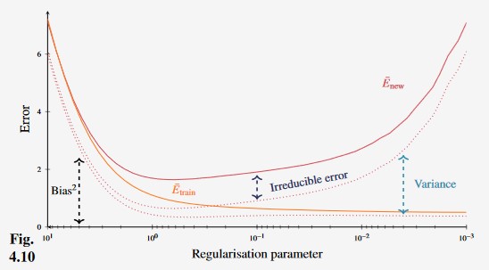
    Figure 8 - Effect of regularisation on error in polynomial regression model.

• From the figure above, we can see that for this particular problem the optimal value of $\lambda$ occurs at around 0.7, where $\overline{E}_\text{new}$ attains its minimum value.

Connections between Bias, Variance and the Generalisation Gap

• Bias and variance are theoretically well-defined but hard to determine the value of in practice (as they are defined in terms of probability distribution $p({\bf{x}},y)$)

• In practice, can have an estimate of the generalisation gap (e.g., as $E_\text{hold-out}-E_\text{train})$ whereas bias and variance require additional tools to estimate.

• Consider regression problem in which squared error is used as both error and loss function

  • Additionally, assume that a global minimum has been found during training.

$$\sigma^2+\text{bias}^2 =\mathbb{E}_\star[(\overline{f}({\bf{x}_\star})-y_\star)^2]\\ \approx\frac{1}{n}\sum_{i=1}^{n}(\overline{f}({\bf{x}}_i)-y_i)^2\\ \ge \frac{1}{n}\sum_{i=1}{n}(\hat{y}({\bf{x}}_i;\mathcal{T})-y_i)^2=E_\text{train}\tag{4.22}$$

• We approximate the expected value by a sampling average using the training data points.
• If we assume that $\hat{y}$ can possibly be $\overline{f}$, together with the assumption of having the squared error as a loss function and the learning of $\hat{y}$ always finding the global minimum, we have the inequality given in the next step.
• Remember that $\overline{E}_\text{new}=\sigma^2+\text{bias}^2+ \text{variance}$, and allow $\overline{E}_\text{new}-E_\text{train}=\text{generalisation gap}$ gives the following:

$$\text{generalisation gap}\overset{\gt}{\approx} \text{variance}\tag{4.23a}$$

$$E_\text{train}\overset{\gt}{\approx}\text{bias}^2+\sigma^2 \tag{4.23b}$$

• In practice, the assumptions don’t always hold.
• Can deal with this through using bagging (ensemble methods) which will be discussed in Chapter 7

Additional Tools for Evaluating Binary Classifiers

• Define some tools for binary classification problem with imbalanced or asymmetric problems
• Consider the binary classification problem in which 90% of the samples belong to class A and 10% to class B.
  • If we evaluate accuracy just using a single acc value, we can gain 90% accuracy just by always predicting class A.
  • We have to look more closely at the types of errors made by the model
• Using a classifier often involves applying some adjustable threshold to make the decision of which class to choose (as in Logistic Regression)
  • If we change this threshold, we are likely to see a change in the classification performance.

Confusion Matrix and ROC Curve

• Confusion Matrix a table that breaks down a comparison of the class predictions vs true class values from training data.
• In the binary case, we can have True Positive, True Negative, False Positive and False Negative
• By separating the predictions into four groups dependent on $y$, the actual output and $\hat{y}$ (the predicted output from the classifier) we can construct the following confusion matrix for the classification problem.

P(N)$ denotes total number of positive (negative) examples in the dataset $P^*(N^*)$ denotes the total number of positive (negative) predictions made by the model. - For asymmetric problems, important to distinguish between False Positive (Type I) and False Negative (Type II) error - Ideally, both types of errors should be 0, but there is typically a tradeoff between these two errors. - The tradeoff between FP and FN can be changed by tuning a decision threshold $r$. - Some of the terminology associated with confusion matrices include: $$\text{recall}=\frac{TP}{P}=\frac{TP}{TP+FN}

$$\text{precision}=\frac{TP}{P^*}=\frac{TP}{TP+FP}$$

• Other common terms associated with Confusion Matrices are given below

Recall: How much of the positive data points are correctly predicted as positive Precision: Ratio of TP are among those predicted positive ROC (Receiver Operating Characteristics): Plotting the ROC curve can be useful in comparing classifiers with different threshold values $r$.

• Plot true positive rate $FP/N$ over false positive rate $FP/N$ for all $r\in[0,1]$$

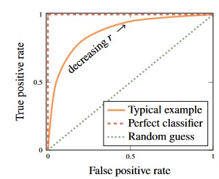
Figure 9 - ROC Curve for Classifier

• Observe that the perfect classifier (red dotted line) touches the top left corner of the plot.

  • This is in contrast to a classifier that gives random guesses - this gives a straight diagonal line

• We can use ROC-AUC (Area under the ROC curve) to summarise the plot

  • A perfect classifier has ROC-AUC=1 and a classifier that assigns random guesses to have ROC-AUC=0.5

• We can use the precision-recall curve for imbalanced problems.

A problem is:

• Imbalanced if the vast majority of the data-points belong to one class (typically, the negative class)
  • The imbalance implies that a (useless) classifier which always predicts $\hat{y}({\bf{x}})=-1$ will score very well in terms of misclassification rate

• Confusion matrix offers good opportunity to inspect FPs and FNs
• Can also use measures such as misclassification rate in balanced problems to summarise this into a single score.
• For imbalanced problems where the negative class is the most common class, the $F_1$ score is better
  • However, $F_\beta$ score is preferred as $F_1$ doesn’t consider the fact that one type of error is considered to be more serious than another
  • $F_\beta$ considers recall to be $\beta$ times more important as precision

$$F_\beta = \frac{(1+\beta)^2\cdot\text{precision}\cdot\text{recall}}{\beta^2\cdot\text{precision}+\text{recall}}$$

• ROC may be misleading for imbalanced problems and so precision-recall curve

Figure 10 - Precision-Recall Curve for Binary Classification Problem. Precision-Recall curves are good for imbalanced classification problems.