Lindholm et al, Chapter 5

Learning Parametric Models

Principles of Parametric Modelling

• A linear regression model is denoted by

$$y=f_\theta({\bf{x}})+\varepsilon\tag{5.1}$$

• Introduced explicit dependence on the parameters $\theta$ in the notation to emphasise that the equation should be viewed as a model of the true input-output relationship.
• For the linear regression model, two key assumptions were made:
  • Function $f_\theta$ assumed to be linear in model parameters, $f_\theta({\bf{x}})=\theta^T{\bf{x}}$.
  • Noise assumed to be of Gaussian distribution $\varepsilon~\mathcal{N}(0,\sigma_\varepsilon^2)$
• Both of these assumptions can be relaxed - first consider relaxing the first assumption
  • Let $f(\cdot)$ be some function that is adaptable to training data, by letting the function depend on model parameters $\theta$ learned from the training set.
• We can use this to transform logistic regression model into a non-linear model by using $f_\theta$

$$g({\bf x}) = \frac{e^{f_\theta({\bf x})}}{1+e^{f_\theta({\bf x})}}\tag{5.3}$$

• Having specified this family of models, we want to learn the parameters $\theta$ from the training data.
• For parametric models, this learning objective is typically formulated as an optimisation problem, denoted:

$$\hat\theta=\arg\min_\theta\underbrace{\frac1n \sum_{i=1}^{n} \overbrace{L(y_i, f_\theta({\bf x_i}))}^{\text{loss function}}}_{\text{cost function } J(\theta)}$$

• Minimise a cost function defined as average of some (user-chosen) loss function evaluated training data.
  • In some cases, can compute the solution exactly (e.g. linear regression, closed-form solution)
  • Most cases require numerical optimisation methods (e.g. gradient descent)
• We really want to minimise $E_\text{new}$ but this error is unknown to us.
• With this concept in mind, we make the following observations:
  • The cost function $J(\theta)$ is computed based on the training data, and is subject to the noise in the data. Therefore, it is not meaningful to optimise $J(\theta)$ with greater accuracy than the statistical accuracy in the estimate.
  • Loss function $\ne$ error function - The error function used should not be the same as the los function - this is said to create models that are able to generalise better. In addition to this, we can choose loss functions that make the optimisation problem easier to solve, or make the model have favourable properties (e.g., make the model less computationally demanding to use in production)
  • Early Stopping is sometimes useful as the end-point of the optimisation isn’t necessarily the set of parameters with lowest $E_\text{new}$.
  • Explicit Regularisation is performed by modifying the cost function by adding a term independent of the training data - we want to find the simplest set of parameters, so we penalise large parameter values.

Loss Functions and Likelihood-Based Models

• Different loss functions give rise to models with different solutions ($\hat\theta$)
  • Different loss functions will be optimal for different problems.
• Certain combinations of models and loss functions have been given certain names:
  • Linear Regression Linear-in-the-parameter models, squared error loss function.
  • Support Vector Classification Linear-in-the-parameters model, hinge loss
• Want to create models that are robust (to outliers in the data).
  • If outliers have minor impact on learned model, say loss function is robust.
  • Important in models created using data contaminated with outliers.

Loss Functions for Regression

• In Chapter 3, introduced squared error loss, which is the default choice for linear regression as it means that the model has a closed-form solution.

$$L(y, \hat y) = (\hat y - y)^2 \tag{5.6}$$

• Another choice is the absolute error loss which is more robust to outliers as it grows more slowly for large errors.

$$L(y,\hat y)=|\hat y - y | \tag{5.7}$$

• This can be justified using the concept of maximum likelihood estimation, just like with the squared error loss
  • Consider that the error has a Laplace distribution $\varepsilon ~\mathcal{L}(0, b_\varepsilon)$
• It is sometimes argued that the squared error loss is a good choice because it penalises small errors ($\varepsilon < 1$) less than linearly.
  • Furthermore, Gaussian distribution appears (at least approximately) quite often in nature
• However, the quadratic shape in nature is the reason for its non-robustness
• Therefore, Huber loss proposed as a hybrid between absolute loss and squared error loss

$$L(y,\hat y) = \begin{cases} \frac 12 (\hat y - y)^2 & \text{ if } |\hat y - y| < 1, \\ |\hat y - y| - \frac12 & \text{ otherwise.} \end{cases} \tag{5.8}$$

• Another extension to the absolute error is the $\epsilon$-insensitive loss, which places a tolerance of width $2\epsilon$ around the observed value $y$ and behaves like the absolute error loss outside of this region.
  • The robustness properties of the $\epsilon$-insensitive loss are very similar to that of absolute error loss
  • This is useful for Support Vector Regression in Chapter 8.

$$L(y,\hat y) = \begin{cases} 0 & \text{ if } |\hat y - y| < \epsilon, \\ |\hat y - y| - \epsilon & \text{ otherwise.} \end{cases} \tag{5.9}$$

Loss Functions for Binary Classification

• An intuitive loss for binary classification is the misclassification loss

$$L(y,\hat y)=\mathbb{I}\lbrace\hat y \ne y\rbrace =\begin{cases}0&\text{if }\hat y = y \\ 1 & \text{if }\hat y \ne y\end{cases}\tag{5.10}$$

• Although this is the ultimate goal, it is rarely used in training
  • Different loss functions can lead to models that generalise better form the training data.
  • We want to maximise the distance of between the decision boundary and each class to ensure better generalisation ability.
  • To do this, we can formulate the loss function not just in terms of hard class predictions, but predicted class probability (or some other continuous quantity used to compute the class prediction)
  • Furthermore, misclassification loss is difficult to optimise from a numerical optimisation perspective since the gradient is zero everywhere (except where it is undefined).
• For a binary classifier that predicts conditional class probabilities $p(y=1|{\bf x})$, in terms of a function $g({\bf x})$ the cross-entropy loss is a natural choice:

$$L(y, g({\bf x})) = \begin{cases}\ln g({\bf x}) & \text{ if } y=1 \\ \ln (1 - g({\bf x})) & \text{if y=-1}\end{cases}\tag{5.11}$$

• Many binary classifiers $\hat y({\bf x})$ can be constructed by thresholding some real-valued function $f({\bf x})$ at 0. That is, we write the class prediction:

$$\hat y ({\bf x}) = \text{sign}\lbrace f ({\bf x}) \rbrace \tag{5.12}$$

• Logistic regression can be brought into this form by simply using $f({\bf x})=\theta^T{\bf x}$ as shown in Equation 3.39.
• For functions of this form, the decision boundary is given by the values of $\bf x$ for which $f({\bf x})=0$.
• The margin can be viewed as a measure of certainty in a prediction, where data points with small margins (not necessarily in the sense of Euclidean distance) are close to the decision boundary.
• We can define loss functions for binary classification in terms of the margin by assigning small loss to positive margins (correct classifications) and large loss to negative margins (incorrect classifications).
• Logistic loss (Equation 3.34) can be re-formulated as:

$$L(y \cdot f({\bf x})) = \ln (1 + \exp (-y \cdot f({\bf x}))) \tag{5.13}$$

• In this equation, the linear logistic regression model corresponds to $f({\bf x}) = \theta^T{\bf x}$
  • Note that in this arrangement, we have lost the notion of a class probability estimate, and only have a hard prediction once again.
• The misclassification loss can also be re-formulated in terms of the margin:

$$L(y \cdot f({\bf x})) = \begin{cases}1&\text{if } y \cdot f({\bf x}) < 0, \\ 0, & \text{otherwise}\end{cases} \tag{5.14}$$

• Another loss function is exponential loss, which is defined as:

$$L(y\cdot f({\bf x}))=\exp(-y\cdot f({\bf x}))\tag{5.15}$$

• We can also define hinge loss, which is defined as:

$$L(y\cdot f({\bf x}))=\begin{cases}1-y\cdot f({\bf x})&\text{if }y\cdot f({\bf x})\le 1\\0&\text{otherwise}\end{cases}\tag{5.16}$$

• One downside of the hinge loss function is that it is not a strictly proper loss function - it is not possible to interpret the learnt classification model probabilistically when using this loss.
  • To remedy this, consider using the squared hinge loss, which is less robust than hinge loss.

$$L(y\cdot f({\bf x})) = \begin{cases}(1-y\cdot f({\bf x}))^2 &\text{for } y \cdot f({\bf x})\le 1\\0&\text{otherwise}\end{cases}\tag{5.17}$$

• An alternative to this is the Huberised squared hinge loss

$$L(y\cdot f({\bf x})) = \begin{cases} -4y\cdot f({\bf x}) &\text{for } y \cdot f({\bf x}) \le -1 \\ (1 - y \cdot f({\bf x}))^2 & \text{for } -1 \le y \cdot f({\bf x}) \le 1 \text{(squared hinge loss)} \\ 0 & \text{otherwise} \end{cases}\tag{5.18}$$

• When learning models for imbalanced or asymmetric problems, it is possible to modify the loss function to account for imbalance/asymmetry.
  • For example, misclassification loss can be modified to penalise that not predicting $y=1$ correctly is a “C times more severe mistake” than not prediction $y=-1$ correctly, the misclassification loss can be modified into Equation 5.19 below
  • A similar effect can be achieved by duplicating all positive training data points $D$ times in the training data instead of modifying the loss function.

$$L(y,\hat y)=\begin{cases} 0 & \text{if} \hat y = y \\ 1 & \text{if } \hat y \ne y \text{ and } y = -1 \\ C & \text{if } \hat y \ne y \text{ and } y = 1 \end{cases}\tag{5.19}$$

Multi-Class Classification

• Cross-entropy loss is easy to generalise to multi-class classification as done in Chapter 3
• Generalisation of other loss functions requires generalising the concept of a margin to the multi-class case.
  • Another alternative is to re-formulate the problem as several binary problems - approach taken in the textbook.

Likelihood-Based Models and the Maximum Likelihood Approach

• Maximising the likelihood is equivalent to minimising cost function based on negative log-likelihood loss

$$J(\theta) = -\frac 1n \sum_{i=1}^{n} \ln p(y_i | {\bf x}_i ; \theta)$$

• In all cases where we have a probabilistic model of conditional distribution $p(y|{\bf x})$ the negative log-loss likelihood is a plausible loss function

• For classification problem, this is simple as $p(y|{\bf x})$ corresponds directly to a probability vector over the $M$ classes

  I have ignored a bunch of content here for the sake of time

Regularisation

• A useful tool for avoiding overfitting if a model is too flexible.
• In a parametric model, the idea of regularisation is to “keep the parameters $\hat\theta$ small unless the data really convinces us otherwise”.
• There are many ways to implement this, distinguish between explicit and implicit regularisation:

L2 Regularisation

Also known as Tikhonov regularisation, weight decay, ridge regression, or shrinkage

• L2 regularisation is a form of explicit regularisation, where we add a penalty term to the cost function that penalises large values of the parameters $\theta$.

$$\hat\theta=\arg\min_\theta\frac 1n || {\bf X}\theta-{\bf y}||_2^2 + \lambda ||\theta||_2^2 \tag{5.22}$$

• By choosing the regularisation parameter $\lambda \ge 0$, a trade-off between the original cost function (fitting training data as well as possible) and the regularisation term (keeping parameters $\hat\theta$ close to 0) is mad.e
• In setting $\lambda=0$, the least squares problem is recovered, whereas with $\lambda\rightarrow\infty$, all parameters will be forced to 0.
  • Optimal values can be found via cross-validation
• Can derive version of normal equations for L2 regularisation:

$$({\bf X}^T{\bf X} + n \lambda {\bf I}_{p+1})\hat{\bf\theta} = {\bf X}^T {\bf y}\tag{5.23}$$

• In the equation ${\bf I}_{p+1}$ is the $(p+1)\times(p+1)$ identity matrix.
• For $\lambda>0$ the matrix ${\bf X}^T{\bf X} + n \lambda {\bf I}_{p+1}$ is always invertible, and the solution is given by:

$$\hat{\bf\theta}=({\bf X}^T {\bf X} + n \lambda {\bf I}_{p+1})^{-1} {\bf X}^T {\bf y} \tag{5.24}$$

• This reveals another motivation for using $L^2$ regularisation for linear regression - when ${\bf X}^T{\bf X}$ is non-invertible, no unique solution exists, however, the regularisation term will ensure that a unique solution exists.

L1 Regularisation

• With L1 regularisation, the penalty term $||\theta||-1$ is added to the cost function.
  • This added penalty term is the L1 norm of the parameter vector $\theta$ (i.e., sum of absolute value of parameters).
• The L1 regularised cost function for linear regression is

$$\hat\theta=\arg\min_\theta\frac 1n || {\bf X}\theta - {\bf y}||_2^2 + \lambda ||\theta||_1 \tag{5.25}$$

• No closed-form solution that exists, but can create efficient numerical optimisation algorithm
• L1 regularisation pushes all parameters toward small values (but not necessarily zero)
• Tends fo favour sparse solutions

Implicit Regularisation

• There are alternative ways to achieve a similar effect without explicitly modifying the cost function
• One way to do this is early stopping - applicable to any method that is trained using iterative numerical optimisation.
• This amounts to stopping the optimisation before it has reached the minimum of the cost function
• Can be implemented by setting aside some hold-out validation data and computing $E_\text{hold-out}$ after each iteration.
  • Observed that $E_\text{hold-out}$ will decrease initially, but eventually reaches a minimum and starts to increase again.
• The optimisation is aborted at the point when $E_\text{hold-out}$ reached its minimum.

Parameter Optimisation

• Want to find minimum or maximum of objective function.
• There are two ways optimisation is used in ML:
  • Training a model by minimising the cost function with respect to model parameters $\theta$. The objective function in this case is $J(\theta)$, and optimisation variables to model parameters $\theta$.
  • Tuning hyper parameters such as $\lambda$, such as using hold-out validation dataset. The objective function is the validation error and the optimisation variables is the hyper parameters.
• Optimisation is easier for convex objective functions - take some time to consider whether we can re-formulate a non-convex optimisation problem into a convex one.
  • The most important property of convex functions is that they have a unique global minimum, and no other minima.
• When closed form solutions don’t exist, we must use (iterative) numerical techniques for solving.
• For L1 regularised linear regression, but it turns out coordinate descent is a good approach for this problem.

Gradient Descent

Useful when we don’t have a closed-form solution but we have access to the value of the objective function and its derivative (gradient).

• Can be used for learning the parameter vectors $\theta$ of high-dimension when the objective function $J(\theta)$ is simple enough that we can compute its gradient.
  • We can potentially also use Gradient Descent for hyperparameter optimisation
• Assume that the gradient of the cost function $\nabla_\theta J(\theta)$ exists for all $\theta$.
  • Note that $\nabla_\theta J(\theta)$ is a vector of the same dimension as $\theta$, which describes the direction in which $J(\theta)$ increases.
• From this, we obtain $-\nabla_\theta J(\theta)$ which is the direction in which $J(\theta)$ decreases
• If we take a small step in the direction of negative gradient, this will reduce the value of the cost function

$$J(\theta-\gamma\nabla_\theta J(\theta)) \le J(\theta) \tag{5.30}$$

• If $J(\theta)$ in convex, the inequality in Equation 5.30 is strict except at the minimum (where the derivative is zero)
• This suggests that if we have $\theta^{(t)}$ and want to select $\theta^{(t+1)}$ such that Equation 5.30 holds true, we should use the following equation, with some $\gamma>0$.

$$\text{update }\theta^{(t+1)} = \theta^{(t)} - \gamma\nabla_\theta J(\theta^{(t)}) \tag{5.31}$$

• The Gradient Descent Algorithm is as follows:

Input: Objective function $J(\theta)$, initial $\theta^{(0)}$, learning rate $\gamma$

Result: $\hat\theta$

1. Set $t=0$
2. while $||\theta^{(t)} - \theta^{(t-1)}$ not small enough do
3.  |   Update $\theta^({t+1})\leftarrow \theta^{(t)} -\gamma\nabla_\theta J(\theta^{(t)})$
4.  |   Update $t\leftarrow t+1$
5. end
6. return $\hat\theta\leftarrow\theta^{(t+1)}$

• When using this algorithm in practice, we do not know $\gamma$ which determines how big the $\theta$ step is at each iteration

  • It is possible to formulate the selection of $\gamma$ as an internal optimisation problem that is solved at each iteration (a “line search problem”)
  • Consider the simpler solution where consider $\gamma$ to be a constant chosen by the user.
  • In this case, $\gamma$ is viewed as a hyperparameter, called the learning rate or step size, and the optimal value depends on the shape of the cost function.

  

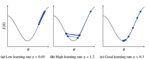
  Figure 5.7 - Effect of learning rate on gradient descent. (Left) Too high learning rate (Middle) Too high learning rate (Right) Good learning rate.

• Can see in Fig 5.7, the effect of different learning rates.

  • If the cost function values are getting worse or oscillating wildly, decrease the learning rate
  • If the learning rate fairly constant and only slowly decreasing, increase the learning rate.

• No guarantees about convergence with gradient descent, as a bad choice of $\gamma$ will break the method.

• With the right choice of learning rate, the value of $J(\theta)$ will decrease fo each iteration until a point with zero gradient is found.

  • However, not necessarily a minimum but could be a maximum or saddle point in the objective function.
  • In non-convex problems with multiple minima, we cannot expect gradient descent to find the global minimum
  • Initialisation is usually critical for determining which minimum is found.

• Good practice to run the optimisation multiple times with different training initialisations.

  • However for large models, this can be computationally expensive, so can use heuristics and tricks to find a good initialisation point

Second-Order Gradients

Omitted as not really covered in the lectures -> not relevant

Optimisation with Large Datasets (SGD)

• With large values of $n$ (samples in the dataset), we can expect that the gradient computed for the first half of the dataset to be almost identical to the gradient computed for the second half.
• Consequently, might be a waste of time to compute the gradient over the entire dataset at each iteration of gradient descent.
• Instead, we can compute the gradient based on the first half of the training set, update the parameters according to the gradient descent method and and then compute the gradient for the new parameters based on the second half of the training data.

$$\theta^{(t+1)} = \theta^{(t)} - \gamma \frac{1}{n/2} \sum_{i=1}^{\frac n2} \nabla_\theta L({\bf }_i, {\bf y}_i, \theta^{(t)}) \tag{5.37a}$$

$$\theta^{(t+2)} = \theta^{(t+1)} - \gamma \frac{1}{n/2} \sum_{i=\frac{n}{2}+1}^{n} \nabla_\theta L({\bf }_i, {\bf y}_i, \theta^{(t+1)}) \tag{5.37b}$$

• Utilising Equation 5.37 requires half the computation compared to the two parameter updates of conventional gradient descent.
• We can further extend this idea into subsampling with even fewer data points used in the gradient computation.
• Call a sub-sample of the data a mini-batch which can typically contain $n_b \in [10, 100, 100]$ samples.
  • One complete pass through the training data is called an epoch, and consists of $n/n_b$ iterations.
• Note: When using mini-batches, it is important to ensure that the mini-batches are balanced and representative of the entire dataset.
  • Mini-batches should be formed randomly - can do this by shuffling the data and dividing into mini-batches.
  • After completing one epoch, perform shuffling of the training data and do another pass through the dataset.
• This idea of gradient descent with mini-batches is called stochastic gradient descent and is summarised in the pseudocode shown below:

Stochastic Gradient Decent Pseudocode

Input Objective Function $J(\theta)=\frac 1n \sum_{i=1}^n L({\bf x}_i, {\bf y}_i, \theta)$, initial $\theta^{(0)}$, learning rate $\gamma$Result $\hat\theta$

1. Set $t\leftarrow 0$
2. while convergence criteria not met do
3.  |   for $i\in\{1,2,\dots,E\}$ do
4.  |   |   Randomly shuffle the training data $\lbrace {\bf x}_i, y_i \rbrace_{i=1}^n$
5.  |   |   for $j\in\{1,2,\dots,\frac{n}{n_b}\}$ do
6.  |   |   |   Approximate the gradient using the mini-batch $\lbrace({\bf x}_i, {\bf y}_i)\rbrace_{i=(j-1) n_b + 1}^{jn_b}, \hat{\bf d}^{(t)} \sum_{i=(j-1)n_b + 1}^{jn_b} \nabla_\theta L({\bf x}_i, y_i, \theta^{(t)})$
7.  |   |   |   Update $\theta^{(t+1)} \leftarrow \theta^{(t)} - \gamma^{(t)} \hat{\bf d}^{(t)}$
8.  |   |   |   Update $t\leftarrow t + 1$
9.  |   |    end
10.  |    end
11. end
12. return $\hat\theta\leftarrow\theta^{(t-1)}$

• Stochastic Gradient Descent is widely used, with different variants for different purposes.

Learning Rate and Convergence for SGD

• Standard gradient descent converges if the learning rate is wisely chosen and constant (since the gradient is zero at the minimum).

• For SGD, cannot obtain convergence with a constant learning rate - we only obtain an estimate of the true gradient, and this estimate will not necessarily be zero at the minimum of the objective function (might be considerable amount of noise in the gradient estimation due to subsampling)

• SGD with constant learning rate will not converge toward a point, but continue to “wander around” somewhat randomly.

• For the gradient descent method to work, also require that the estimate is unbiased - if unbiased, will on average step in the right direction toward the optimum.

• By decreasing the learning rate over time, the parameter updates will become smaller and smaller.

• Start with $t=0$ and a fairly high learning rate $\gamma^{(t)}$ and decay as $t$ increases.

There was other content here, but I have decided to omit it because it’s taking too much time

Hyperparameter Optimisation

• Simplest way optimiser hyper-parameters is to perform a “grid search”.
• Very computationally inefficient especially for parameter vectors with high dimensionality.
  • This is fine for problems with low-dimensional hyper-parameters but grows quickly with the number of hyper-parameters.
• If we consider points for which the objective function has already been evaluated as a training dataset, we can use a regression method to learn a model for the objective function.
  • This model can be used to predict where to evaluate the objective function next.