Lindholm et al, Chapter 6

Neural Networks and Deep Learnings

• Can effectively stack multiple parametric models to construct a new model that is able to describe more complex input/output relationships than linear or logistic models are able to.

The Neural Network Model

• We can describe the non-linear relationship between input variables and outputs in its prediction form as:

$$\hat\theta=f_\theta(x_1, \dots, x_p)\tag{6.1}$$

• where $f$ is a function parameterised by $\theta$, which can be parameterised in many ways.
• The general strategy for neural networks is to use several layers of regression models and non-linear activation functions.

Generalised Linear Regression

• Begin with description of a neural network with the linear regression model:

$$\hat y = W_1 x_1 + W_2 x_2 + \cdots + W_p x_p + b \tag{6.2}$$

• Here, denote parameters by the weights $W_1, \dots, W_p$ and the offset term (bias) $b$.

  

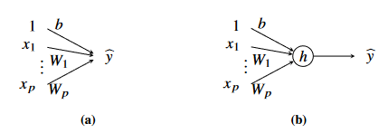
  Figure 1 - (a) Graphical illustration of linear regression model and (b) generalised linear regression model. In (a), the output is the sum of all terms, b and the weighted inputs. In (b), the output is the sum of all terms, b and the weighted inputs passed through a non-linear activation function h

• Each input variable is represented by a node, and each parameter $W_j$ by a link.

• The output $\hat y$ is the sum of all terms $W_j x_j$ plus the bias term $b$.

  • By convention, use constant value 1 to as the input variable corresponding to the bias term.

• To describe the non-linear relationship between input and output, introduce a non-linear function called the activation function $h:\mathbb{R}\rightarrow \mathbb{R}$.

  • With this notation, the generalised linear regression model is denoted as

$$\hat y = h(W_1 x_1 + W_2 x_2 + \cdots + W_p x_p + b) \tag{6.3}$$

• Common activation functions are the Logistic Function and the Rectified Linear Unit.
• The generalised linear regression model in Equation 6.3 above is not capable of describing complex relationships.
  • Make use of several parallel generalised linear regression models to create a layer, and stack these layers in a sequential construction
  • This will result in a deep neural network.

Two-Layer Network

• In Equation 6.3, the output $\hat y$ is constructed by a single scalar regression model.
• To increase its flexibility and turn it into a two-layer network, we let its output be sum of $U$ such generalised linear regression models, each of which has its own set of parameters.
• The parameters for the $k$th regression model are $b_k, W_{k1}, \dots, W_{kp}$ and we denote its output by $q_k$.

$$q_k = h(W_{k1} x_1 + W_{k2} x_2 + \cdots + W_{kp} x_p + b_k), \quad\quad k=1,\dots,U \tag{6.4}$$

• These intermediate outputs are known as hidden units, since they are not the output of the whole model. The $U$ different hidden units $\{q_k\}_{k=1}^U$ instead act as input variables to an additional linear regression model.

$$\hat y = W_1 q_1 + W_2 q_2 + \cdots W_U q_U + b \tag{6.5}$$

• To distinguish the parameters in Eq 6.4 and 6.5, add superscripts $(1)$ and $(2)$ respectively.

$$\begin{align*} q_1 &= h(W_{11}^{(1)} x_1 + W_{12}^{(1)} x_2 + \cdots W_{1\ p}^{(1)} + b_1^{(1)}),\\ q_2 &= h(W_{21}^{(1)} x_1 + W_{22}^{(1)} x_2 + \cdots W_{2\ p}^{(1)} + b_2^{(1)}),\\ \vdots\\ q_U&=h(W_{U1}^{(1)} x_1 + W_{U2}^{(1)} x_2 + \cdots W_{U\ p}^{(1)} + b_U^{(1)}),\\ \end{align*} \tag{6.6a}$$

• Then out final model is denoted as

$$\hat{y}=W_1^{(2)}q_1 + W_2^{(2)}q_2 + \cdots + W_U^{(2)} + b^{(2)} \tag{6.6b}$$

• This notation can be written more compactly using matrix notation, where the parameters in each layer are stacked in a weight matrix $\bf W$ and an offset vector $\bf b$ as:

$$\begin{align*} {\bf{W}}^{(1)} &= \begin{bmatrix} W_{11}^{(1)} & \cdots & W_{1p}^{(1)}\\ \vdots & & \vdots \\ W_{U1}^{(1)} & \cdots & W_{U p}^{(1)}\\ \end{bmatrix}, \ \ \ \ &&{\bf{b}}^{(1)}= \begin{bmatrix} b_1^{(1)}\\ \vdots\\ b_U^{(1)} \end{bmatrix}, \\ W^{(2)} &= \begin{bmatrix} W_1^{(2)} & \cdots & W_U^{(2)} \end{bmatrix}, &&{\bf{b}}^{(2)} = \begin{bmatrix} b^{(2)} \end{bmatrix}, \end{align*} \tag{6.7}$$

• With this, the full model is written as

$$\begin{align} &{\bf{q}} = h({\bf{W}}^{(1)} x + {\bf{b}}^{(1)}), \tag{6.8a} \\ &\hat{y}={\bf{W}}^{(2)} {\bf{q}} + {\bf{b}}^{(2)}, \tag{6.8b} \end{align}$$

• In this equation, the components in $\bf x, q$ have been stacked as ${\bf x}=\begin{bmatrix} x_1& \dots& x_p\end{bmatrix}^T$ and ${\bf q}=\begin{bmatrix} q_1& \dots& q_U\end{bmatrix}^T$.
• Additionally, the activation function in this equation acts element-wise across the inputs.
• The weight matrices and offset vectors are the parameters of the model, which can be compiled as a single vector (in the 2-layered perceptron shown above):

$$\def\vec{\text{vec}} \def\W {{\bf{W}}} \def\b {{\bf{b}}} \theta=\begin{bmatrix} \vec(\W^{(1)})^T & \vec(\b^{(1)})^T & \vec(\W^{(2)})^T & \vec(\b^{(2)})^T \end{bmatrix}$$

Deep Neural Networks

• Enumerate layers with index $l\in\{1,\dots,L\}$, where $L$ is the total number of layers.
• Each layer is parameterised by a weight matrix ${\bf W}^{(l)}$ and an offset vector ${\bf b}^{(l)}$.
• Multiple layers of hidden units denoted by ${\bf q}^{(l)}$.
• Each layer consists of $U_l$ hidden units ${\bf q}^{(l)} = \begin{bmatrix} q_1^{(l)} & \dots & q_{U_l}^{(l)}\end{bmatrix}^T$.
  • Note that in this equation, $U_1,\dots,U_{L-1}$ can be different across the various layers.
• Each layer maps a hidden layer ${\bf q}^{(l-1)}$ to the next hidden layer ${\bf q}^{(l)}$ according to the following equation:

$${\bf{q}}^{(l)} = h({\bf{W}}^{(l)} {\bf{q}}^{(l-1)} + {\bf{b}}^{(l)}) \tag{6.10}$$

• A DNN of $L$ layers is then written as:

$$\def\q{{\bf q}} \def\W{{\bf W}} \def\b{{\bf b}} \begin{align*} \q^{(1)} &= h(\W^{(1)} x + \b^{(1)}), \\ \q^{(2)} &= h(\W^{(2)} \q^{(1)} + \b^{(2)}),\\ &\ \ \ \vdots\\ \q^{(L-1)} &= h(\W^{(L-1)} \q^{(L-2)} + \b^{(L-1)}),\\ \end{align*} \tag{6.11}\\ \hat y = \W^{(L)} \q^{(L-1)} + \b^{(L)}$$

Neural Networks for Classification

• We can use neural networks for classification where we have categorical outputs.
• We can extend neural networks to classification in the same way as linear regression to logistic regression.

$$\text{softmax}({\bf z})\overset\triangle=\frac{1}{\sum_{j=1}^M e^{z_j}}\begin{bmatrix}e^{z_1}\\ e^{z_2} \\ \vdots \\ e^{z_M}\end{bmatrix} \tag{6.15}$$

• The softmax function now becomes an additional activation function acting on the final layer of the neural network.
• It maps the output of the final layer to a probability distribution over the $M$ classes, $p(y_i=m |{\bf x}_i)$.
  • The output corresponds to the probability that the input corresponds to the $j$th class.
• The input variables to the softmax function are referred to as logits.
• The softmax function is not another layer with parameters, merely as a transformation to the output.

Training a Neural Network

• A neural network is a parametric model and its parameters are found using techniques described in the previous chapter.
• The model parameters are weight matrices and offset vectors

$$\def\vec{\text{vec}} \def\W {{\bf{W}}} \def\b {{\bf{b}}} \theta=\begin{bmatrix} \vec(\W^{(1)})^T & \vec(\b^{(1)})^T & \vec(\W^{(2)})^T & \vec(\b^{(2)})^T \end{bmatrix}$$

• To find suitable values for the parameters $\theta$ we solve an optimisation of the following form:

$$\hat\theta=\arg\min_\theta J(\theta), \quad\quad\text{ where} J(\theta)=\frac 1n \sum_{i=1}^n L({\bf x}_i, {\bf y}_i, \theta)\tag{6.18}$$

Backpropagation

• An algorithm that efficiently computes the cost function and its gradient with respect to all parameters in the neural network
• Cost function and gradient are used in SGD algorithms
• The parameters in this model are all weight matrices and weight vectors

$$\def\W{{\bf{W}}} dW^{(t)} \overset{\triangle}{=} \nabla_{\partial\W^{(l)}} J(\theta) = \begin{bmatrix} \frac{\partial J(\theta)}{\partial\W_{11}^{(l)}} & \cdots & \frac{\partial J(\theta)}{\partial\W_{1,U^{(l-1)}}^{(l)}}\\ \vdots && \vdots \\ \frac{\partial J(\theta)}{\partial \W_{U^{(l)},1}^{(1)}}& \cdots & \frac{\partial J(\theta)}{\partial \W_{U^{(l)},U^{(l-1)}}} \end{bmatrix} \tag{6.22a}$$

$$d{\bf{b}}^{(l)} \overset{\triangle}{=} \nabla_{\partial {\bf{b}}^(l)} J(\theta)=\begin{bmatrix} \frac{\partial J(\theta){\partial b_1}}{\partial b_1^{(l)}}\\ \vdots\\ \frac{\partial J(\theta){\partial b_1}}{\partial b_{U^{(l)}}^{(l)}}\\ \end{bmatrix}$$

• We use these to do our update for gradient descent (Eqn 6.23)

$$\def\W{{\bf{W}}} \def\b{{\bf{b}}} W_{t+1}^{(l)} \leftarrow \W_t^{(l)} - \gamma d\W_t^{(l)},\tag{6.23a}$$

$$\def\W{{\bf{W}}} \def\b{{\bf{b}}} b_{t+1}^{(l)} \leftarrow \b_t^{(l)} - \gamma d\b_t^{(l)},\tag{6.23b}$$

• To compute the gradients efficiently, backpropagation uses Calculus chain rule instead of naively computing the derivatives.
• The gradient with respect to the (total weighted sum of) input signals to the units in a layer $d{\bf{z}}^{(l)}$ and the output signals of units in a layer $d{\bf{q}}^{(l)}$ given in Eq 6.25

$$d{\bf z}\triangleq \nabla_{z^{(l)}} J(\theta) = \begin{bmatrix} \frac{\partial J(\theta)}{\partial z_1^{(l)}}\\ \vdots\\ \frac{\partial J(\theta)}{\partial z_{U^{(l)}}^(l)} \end{bmatrix} \tag{6.25a}$$

$$d{\bf q}^{(l)} \triangleq \nabla_{{\bf{q}}^{(l)}} J(\theta)= \begin{bmatrix} \frac{\partial J(\theta)}{\partial q_1^{(l)}}\\ \vdots\\ \frac{\partial J(\theta)}{\partial q_{U^{(l)}}^{(l)}} \end{bmatrix} \tag{6.25b}$$

• In the backward propagation, compute all gradients $d{\bf z}^{(l)}$ and $d{\bf q}^{(l)}$ for all layers, from layer $L\rightarrow 1$.

• Then, we start calculating the gradients at the output layer, using the derivative of the activation function and $J$ in Eq 6.26.

  • 6.26a describes that for regression problems, the derivative at the end of our MLP which uses squared-error loss is given by:

    $$dz^{(L)} = \frac{\partial J(\theta)}{\partial z^{(L)}} (y-z^{(L)})^2 = -2 (y-z^{(L)}) \tag{6.26a}$$

  • 6.26b describes the derivative for a multi-class classification problem with cross-entropy loss.

    $$dz_j^{(L)} = \frac{\partial J(\theta)}{\partial z^{(L)}} = \frac{\partial}{\partial z^{(l)}}(-z_y^{(L)} + \ln \sum_{k=1}^{M} e^{z_k^{(L)}}) = - \mathbb{I}\lbrace y = j \rbrace + \frac{e^{z_j^{(L)}}}{\sum_{k=1}^{M} e^{z_k^{(L)}}}$$

• The gradients for the weight and bias weights in that layer can be computed, and the gradient signals in the current layer are used to compute the gradients for the previous layer Eq 6.27

$$d{\bf{z}}^{(l)} = d{\bf q}^{(l)} \odot h' ({\bf z}^{(l)}) \tag{6.27a}$$

$$d{\bf{q}}^{(t-1)} = {\bf W}^{(t)T} d({\bf z}^{(l)}) \tag{6.27a}$$

• Note here that $\odot$ denotes the element-wise product and $h'(z)$ is the derivative of the activation function $h(z)$.

  • $h'({\bf{z}})$ acts element-wise on $\bf z$

    

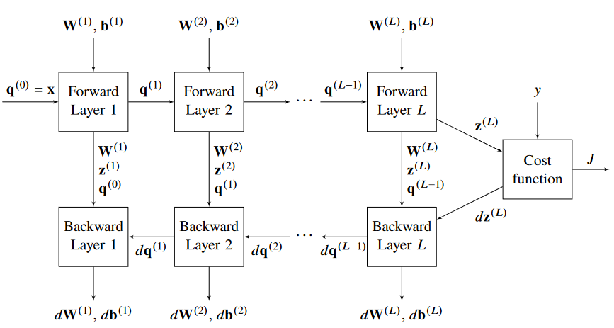
    Figure 5 - Graphical representation of the backpropagation algorithm

• The backpropagation algorithm is given as:

Input:

• Parameters ${\bf{\theta}} = \lbrace {\bf{W}}^{(l)}, {\bf{b}}^{(l)}\rbrace_{l=1}^{L}$
• Activation function $h$
• Data $\bf{X}, y$ with $n_b$ rows where each row corresponds to one data point in the current mini-batch Result: $J(\theta)$, $\nabla_\theta J(\theta)$ of the current mini-batch

1. Forward-Propagation
2. Set ${\bf{Q}}^0\leftarrow \bf{X}$
3. for $l=1,\cdots, L$ do
4.  |   ${\bf{Z}}^{(l)} = {\bf{Q}}^{(l)T} + {\bf{b}}^{(l)T}$
5.  |   ${\bf{Q}}^{(l)} = h({\bf{Z}}^{(l)})$        Do not execute this line for the last layer $l=L$
6. end
7. Evaluate the cost function
8. if Regression problem then
9.  |   $J(\theta)=\frac{1}{n_b} \sum_{i=1}^{n_b} (y_i-Z_i^{(L)})^2$
10.  |   $d{\bf{Z}^{(L)}}=-2({\bf{y}}-{\bf{Z}}^{(L)})$
11. else if Classification problem then
12.  |   $J(\theta) = \frac{1}{n_b} \sum_{i=1}^{n_b} (-Z_{i,y_i}^{(L)} + \ln (\sum_{j=1}^{M} \exp (Z_{ij}^{(L)})))$
13.  |   $dZ_{ij}^{L}=-\mathbb{I}\lbrace y_i=j\rbrace + \frac{\exp (Z_{ij}^{(L)})}{\sum_{j=1}^M \exp(Z_{ij}^{(L)})} \ \ \ \ \forall i,j$
14. Backward Propagation
15. for $l=L,\cdots,1$ do
16.  |   $d{\bf Z}^{(l)}=d{\bf{Q}}^{(l)}\odot h' ({\bf{Z}}^{(l)})$       Do not execute this line for the last layer $l=L$
17.  |   $d{\bf Q}^{(l-1)} = d{\bf{Z}}^{(l)}{\bf{W}}^{(l)}$
18.  |   $d{\bf W}^{(l)} = \frac{1}{n_b} d{\bf{Z}}^{(l)T}{\bf{Q}}^{(l-1)}$
19.  |   $d{\bf b}^{(l)}_j = \frac{1}{n_b} \sum_{i=1}^{n_b} dZ_{ij}^{(l)}\ \ \ \ \ \ \forall j$
20. end
21. $\nabla_\theta J(\theta)=\begin{bmatrix}\text{vec}(d{\bf{W}}^{(1)})^T & d{\bf b}^{(1)T} & \cdots & \text{vec}(d{\bf W}^{(L)})^T & d{\bf b}^{(L)T}\end{bmatrix}$
22. return $J(\theta), \nabla_\theta J(\theta)$

Initialisation

• Training is sensitive to initial parameters as cost functions are usually non-convex.
• Typically initialise all parameters to small random numbers to enable different hidden units to encode different aspects of the data
• If ReLU activation functions used, offset elements $b_0$ are typically initialised to small positive values such that they operate in the non-negative range of ReLU.

Convolutional Neural Networks

• Used for data with grid-like structure, also single-dimension and three-dimensional data
• Each pixel in a greyscale image can be represented as a value in the range [0,1]
• General idea that pixel close together have more in common than pixels far apart.

Convolutional Layers

• Dense / fully connected layer found to be too flexible for images, and might not capture patterns of real importance
  • Models will not generalise and perform well on new data
• Exploit the structure present in images to find a more efficiently parameterised model.
• Uses sparse interactions and parameter sharing
  • Sparse Interactions Most parameters in a corresponding dense layer forced to be equal to zero.
  • Parameter Sharing In a dense layer, each link between input variable and hidden unit is its own unique layer. Instead use the same filter for each pixel in the image.

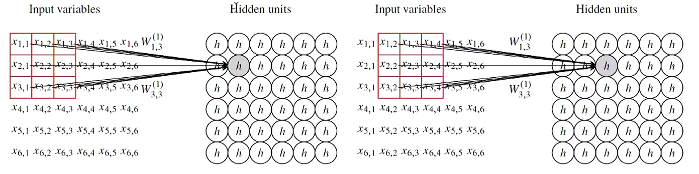
Strided Convolution allows for control over how many pixels in the filter shifts over at each step.

Pooling Layers

• Another way of summarising the information in previous layers can be done by using pooling layers.
• The output from the pooling layer is only dependent on the region of pixels around it.
• Max Pooling takes the maximum value from the region of pixels in the previous layer.
• Average Pooling takes the average value from the region of pixels in the previous layer.

Multiple Channels

• The network in the figure above only has 10 parameters, so one way to extend is to add more channels (by adding multiple kernels), each with their own set of parameters.
• One filter is probably not enough to encode interesting properties in the image.

Full CNN Architecture

• Use convolution layers to perform extract features and then use dense layers for classification or regression.
  • Use softmax to bound sum between [0,1] for classification.

Dropout

• A technique to prevent overfitting in neural networks.
• Training multiple models and averaging predictions is one way to reduce variance (idea behind bagging)
• Bagging comes with problems with NNs - computation time to train, and memory required to store all the parameters.
• Drop-out is like a bagging technique that allows combination of many NNs without needing to train them separately.
• Set random hidden units to 0 (effectively removing them).
• At testing time, remove the drop-out.