Chapter 9 Summary

The Bayesian Idea

• Thus far, learning a parametric model amounts to somehow finding a parameter value $\hat\theta$ that best fits the training data.

• With the Bayesian approach, learning data amounts to finding hte distribution of the parameter values $\theta$ conditioned on the observed training data $\mathcal{T}$ - $p(\theta|\mathcal{T})$

• The prediction is a distribution $p(y_\star|{\bf x_\star} , \mathcal{T})$ instead of a single value.

• With the Bayesian approach, the parameters of any model are consistently treated as being random variables.

• Learning amounts to computing the distribution of $\theta$ conditional on the training data, denoted $p(\theta|{\bf y})$ since we omit $\bf X$.

• The computation is done using joint distribution factorisation and bayes theorem.

• By the laws of probabilities, $p({\bf y})$ can be written as:

$$p({\bf y})=\int p({\bf y}|\theta)p(\theta)d\theta = \int p({\bf y}|\theta)p(\theta) d\theta \tag{9.2}$$

• Training a parametric model amounts to conditioning $\theta$ on $\bf y$ - $p(\theta|{\bf y})$.
• After training, the model can be used to compute predictions - a matter of computing distribution $p(y_\star|{\bf x_\star})$ rather than a point prediction, for a given test input $\bf x_\star$.

$$p(y_\star|{\bf x_\star}) = \int p(y_\star|\theta)p(\theta|{\bf y})d\theta \tag{9.3}$$

• Here $p(y_\star|\theta)$ encodes the distribution of the test data output $y_\star$ in which the corresponding input $\bf x_\star$ is omitted in the notation.
• The other elements involved in the Bayesian approach are traditionally given the names:
  • $p(\theta)$ - prior
  • $p(\theta|{\bf y})$ - posterior
  • $p(y_\star|\theta)$ - posterior predictive (likelihood)

Representation of Beliefs.

• The prior represents our beliefs about a $\theta$ before any data has been observed.

• The likelihood $p({\bf y}|\theta)$ defines how data $\bf y$ relates to the parameter $\theta$

  • Using Bayes theorem, we update the belief about $\theta$ to the posterior $p(\theta | y)$ which also takes the observed data $\bf y$ into account.

• These distributions represent the uncertainty about the parameter $\theta$ before and after observing the data $\bf y$.

• The Bayesian approach is less prone to overfitting when compared to the maximum-likelihood based approach.

  • With the maximum likelihood framework, obtain a single value $\hat\theta$ and use that to make our prediction according to $p(y_\star|\hat\theta)$
  • With the Bayesian distribution, obtained an entire distribution $p(\theta|{\bf y})$ representing the different hypotheses for the value of our model parameters.

• In small datasets, the uncertainty seen the posterior $p(\theta|{\bf y})$ represents how much (or little) can be said about $\theta$ from the presumably limited information in $\bf y$ under the assumed conditions.

• The posterior $p(\theta|{\bf y})$ is a combination of the prior belief $p(\theta)$ and the information about $\theta$ carried by $\bf y$ through the likelihood

  • Without a meaningful prior $p(\theta)$, the posterior $p(\theta|{\bf y})$ is not meaningful either.

Bayesian Linear Regression

• Let $\bf z$ denote a q-dimensional multivariate Gaussian random vector $\bf z = \begin{bmatrix}z_1&x_2&\dots&z_q\end{bmatrix}^T$.
• The multivariate Gaussian distribution is parameterized by a $q$-dimensional mean vector $\bf \mu$ and a $q\times q$ covariance matrix $\bf \Sigma$.

$${\bf\mu}=\begin{bmatrix}\mu_1\\\mu_2\\\vdots\\\mu_q\end{bmatrix}, {\bf\Sigma} = \begin{bmatrix} \sigma_{1}^2&\sigma_{12}&\dots&\sigma_{1q}\\ \sigma_{21} & \sigma_{2}^2 & & \sigma_{2q}\\ \vdots & & & \vdots\\ \sigma_{q1} & \sigma_{q2} & \dots & \sigma_{q}^2 \end{bmatrix}$$

• The covariance matrix is a real-valued positive semidefinite matrix - a symmetric matrix with nonnegative eigenvalues.
• The covariance matrix is positive definite if all eigenvalues are positive.As a shorthand, we write $\bf z \sim \mathcal{N}({\bf \mu}, {\bf \Sigma})$ or $p({\bf z}) = \mathcal{N}({\bf z} ; {\bf \mu}, {\bf \Sigma})$.
• The expected value of $\bf z$ is $\mathbb{E}[{\bf z}] = {\bf \mu}$ and the variance of $z_1$ is $\text{var}(z_1) = \mathbb{E}[(z_1 - \mathbb{E}[z_1])^2]= \sigma_1^2$.
• The covariance between $z_1, z_2$ is $\text{cov}(z_1, z_2) = \mathbb{E}[(z_1 - \mathbb{E}[z_1])(z_2 - \mathbb{E}[z_2])] = \sigma_{12}=\sigma_{21}$.

From Chapter 3, the linear regression model is given by:

$$y=f({\bf x}) + \varepsilon, f({\bf x})=\theta^T{\bf x}, \varepsilon \sim \mathcal{N}(0,\sigma^2)\tag{9.6}$$

$$p(y|\theta)=\mathcal{N}(y;\theta^T{\bf x},\sigma^2) \tag{9.7}$$

• This expression is for one output point $y$, and thus the vector for all training outputs $\bf y$ is denoted as:

$$p({\bf y}|\theta)=\prod_{i=1}^n p(y_i|\theta)=\prod_{i=1}^n\mathcal{N}(y_i;\theta^T{\bf x}_i,\sigma^2) =\mathcal{N}({\bf y};{\bf X}\theta, \sigma^2{\bf I}\tag{9.8}$$

• In the last step, use the fact that $n$-dimensional Gaussian random vector with diagonal covariance matrix is equivalent to $n$ scalar Gaussian random variables.
• With the Bayesian approach, there is also a need for a prior $p(\theta)$ for the unknown parameters $\theta$.
• In Bayesian linear regression, the prior distribution is most often chosen as a linear regression with mean ${\bf\mu}_0$ covariance ${\bf\Sigma}_0$ (for example, ${\bf\Sigma}_0=\sigma^2{\bf I}$)

$$p(\theta)=\mathcal{N}(\theta;{\bf\mu}_0,{\bf\Sigma}_0)\tag{9.9}$$

• The choice of this is motivated by the fact that it simplifies the computation for linear regression.
• We now need to compute the posterior distribution $p(\theta|{\bf y})$

$$\begin{align*} p(\theta|{\bf y})&=\mathcal{N}(\theta;{\bf \mu}_n, {\bf \Sigma}_n) \tag{9.10a} \\ {\bf\mu}_n&={\bf\Sigma}_n \left(\frac{1}{\sigma_0^2} {\bf\mu}_0 + \frac{1}{\sigma^2} {\bf X}^T {\bf y}\right) \tag{9.10b} \\ {\bf\Sigma}_n &= \left(\frac{1}{\sigma_0^2} {\bf I} + frac{1}{\sigma_0^2} {\bf X}^T {\bf X}\right) \tag{9.10c} \end{align*}$$

• From Equation 9.10, we can also derive the posterior prediction for $f({\bf x}_\star)$:

$$\begin{align*} p(f({\bf x_\star} | {\bf y})) &= \mathcal{N}(f({\bf x_\star}); m_\star, s_\star), \tag{9.11a}\\ m_\star&={\bf x}_\star^T {\bf\mu}_n \tag{9.11b}\\ s_\star&={\bf x}_\star^T {\bf\Sigma}_n {\bf x}_\star + \sigma^2 \tag{9.11c} \end{align*}$$

• We can also compute the posterior predictive for $\bf y_\star$

$$p(y_\star | {\bf y}) = \mathcal{N}(y_\star; m_\star, s_\star + \sigma^2) \tag{9.11d}$$

Connection to Regularised Linear Regression

• The main feature of Bayesian approach is that it provides a full distribution $p(\theta|{\bf y})$ for the parameters $\theta$, rather than a single point estimate.
• The MAP estimate and the L2 regularised estimate of $\theta$ are identical for some value of $\lambda$.

The Gaussian Process

• Instead of considering the parameters $\theta$ as random variables, we can consider the function $f({\bf x})$ as a random variable and compute the posterior distribution $p(f({\bf x})|{\bf y})$.

• The Gaussian Process is a type of stochastic process; a generalisation of a random variable.

• Consider the concept of stochastic process to random functions with arbitrary inputs $\lbrace f({\bf x}) : {\bf x} \in \mathcal{X}\rbrace$ where $\mathcal{X}$ denotes the (possibly high-dimensional) input space.

  • With this, the function values $f({\bf x})$ and $f({\bf x'})$ for inputs $\bf x, x'$ are dependent.

• If we expect the function to be smooth (varies slowly), then the function values $f({\bf x})$ and $f({\bf x'})$ should be highly correlated if $\bf x$ and $\bf x'$ are close.

• This generalisation allows us to use random functions as priors for unknown functions in a Bayesian setting.

• Start by making the simplifying assumption that $\bf x$ is discrete and can only take $q$ different values, ${\bf x}_1, {\bf x}_2, \dots, {\bf x}_q$.

  • The function is completely characterised by the vector $\bf f = \begin{bmatrix}f_1&\cdots&f_q\end{bmatrix}^T=\begin{bmatrix}f({\bf x}_1)& \dots& f({\bf x}_q)\end{bmatrix}^T$.
  • We can then model $f({\bf x})$ as a random function by assigning a joint probability distribution to this vector $\bf f$.
  • In the Gaussian process model, this distribution is the multivariate Gaussian distribution, with mean vector $\bf\mu$ and covariance matrix $\bf\Sigma$.

$$p({\bf f}) = \mathcal{N}({\bf f};{\bf \mu,\Sigma})\tag{9.15}$$

• Let us partition ${\bf f}$ into two vectors ${\bf f}_1$ and ${\bf f}_2$ such that $\bf f = \begin{bmatrix} {\bf f}_1 & {\bf f}_2 \end{bmatrix}^T$ and do the same thing for $\bf\mu$ and $\bf\Sigma$:

$$p\left(\begin{bmatrix}{\bf f}_1 \\ {\bf f}_2 \end{bmatrix}\right) =\mathcal{N} \left( \begin{bmatrix}{\bf f}_1 \\ {\bf f}_2 \end{bmatrix}; \begin{bmatrix}{\bf \mu}_1 \\ {\bf \mu}_2 \end{bmatrix}, \begin{bmatrix}{\bf \Sigma}_{11} & {\bf \Sigma}_{12} \\ {\bf \Sigma}_{21} & {\bf \Sigma}_{22} \end{bmatrix} \right) \tag{9.16}$$

• If some elements of $\bf f$, say ${\bf f}_1$, are observed, the conditional distribution for ${\bf f}_2$then we can compute the conditional distribution of the remaining elements ${\bf f}_2$ given ${\bf f}_1$ is given as:

$$p({\bf f}_2|{\bf f}_1) = \mathcal{N}({\bf f}_2;{\bf \mu}_2 + {\bf \Sigma}_{21} {\bf\Sigma}_{11}^{-1}({\bf f}_1-{\bf \mu}_1), {\bf\Sigma}_{22} - {\bf\Sigma}_{21}{\bf\Sigma}_{11}^{-1}{\bf\Sigma}_{12}) \tag{9.17}$$

• The conditional distribution is nothing but another Gaussian distribution (with closed-form expressions for mean and covariance).

  

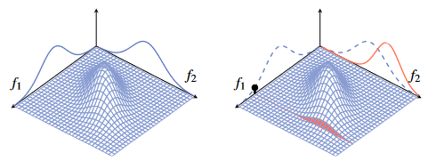
  Figure 1 - Gaussian distribution for random variables f1 and f2 before and after sampling a value.

• In the figure, ${\bf f}_1$ is a scalar $f_1$ and ${\bf f}_2$ is a scalar $f_2$.

• The multivariate Gaussian distribution to the right is now conditioned on an observation of $f_1$ which is reflected on the right side.

  • Both of these Gaussian distributions have the same mean vector and covariance matrix.

• Since ${\bf f}_1$ and ${\bf f}_2$ are correlated according to the prior, the marginal distribution of $f_2$ is also affected by this distribution.

  

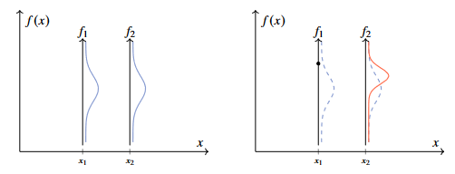
  Figure 3 - Gaussian distribution for random variables f1 and f2 before and after sampling a value.

• In a similar fashion to the figure above, we can plot a six-dimensional Gaussian distribution.

• Assume a positive prior correlation between all elements $f_i$ and $f_j$ which decays with the distance between corresponding inputs $x_i$ and $x_j$.

• We condition the six-dimensional distribution underlying the figure on an observation of $f_4$ for example, producing the following plot:

  

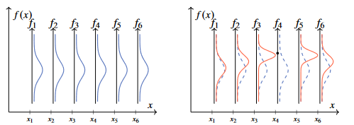
  Figure 4 - A six-dimensional Gaussian distribution conditioned on an observation of $f_4$. Note here that only the marginals in both subplots are plotted.

• The extension of the Gaussian distribution (defined on a finite set) to the Gaussian process (defined on a continuous space) is achieved by replacing the discrete in dex set $\lbrace 1, 2, 3, 4, 5, 6\rbrace$ in the figure above by taking a variable $\bf x$ taking values on a continuous space, for the example the real line.

• We then have to replace the random variables $f_1, f_2, c\dots, f_6$ with a random function (that is, a stochastic process) $f$ which can be evaluated at any $\bf x$ for any $f({\bf x})$.

• In the Gaussian multivariate distribution, $\bf\mu$ is a vector with $q$ components, and $\bf\Sigma$ is a $q\times q$ matrix.

  • Instead of having a separate hyperparameter for each element in this mean vector and covariance matrix in the Gaussian process replace $\bf\mu$ by the mean function $\mu({\bf x})$ into which we can insert any $\bf x$.
  • Likewise, the covariance matrix $\bf\Sigma$ is replaced by the covariance function $\kappa(x,x')$ into which we can insert any pair $\bf x$ and $\bf x'$.

• From this, we can define the Gaussian Process - for any arbitrary finite set of points $\lbrace {\bf x}_1, \dots, {\bf x}_n\rbrace$ it holds that:

$$p\left( \begin{bmatrix} f({\bf x}_1) \\ \vdots \\ f({\bf x}_n) \end{bmatrix}\right) = \mathcal{N}\left( \begin{bmatrix} f({\bf x}_1) \\ \vdots \\ f({\bf x}_n) \end{bmatrix}; \begin{bmatrix} \mu({\bf x}_1) \\ \vdots \\ \mu({\bf x}_n) \end{bmatrix}, \begin{bmatrix} \kappa({\bf x}_1, {\bf x}_1) & \cdots & \kappa({\bf x}_1, {\bf x}_n) \\ \vdots & & \vdots \\ \kappa({\bf x}_n, {\bf x}_1) & \cdots & \kappa({\bf x}_n, {\bf x}_n) \end{bmatrix} \right) \tag{9.18}$$

• With a gaussian process $f$ and any choice of $\lbrace {\bf x}_1, \dots, {\bf x}_n\rbrace$, the vector of value functions $\begin{bmatrix} f({\bf x}_1) & \dots & f({\bf x}_n) \end{bmatrix}^T$ has a multivariate Gaussian distribution.
• Since $\lbrace {\bf x}_1, \dots, {\bf x}_n\rbrace$ can be chosen arbitrarily from the continuous space on which it lives, the Gaussian process defines a distribution for all points on that space.
• For this definition to make sense, $\kappa({\bf x,x'})$ has to be such that a positive semidefinite covariance matrix is obtained for any choice of $\lbrace {\bf x}_1, \dots, {\bf x}_n\rbrace$.
• Let the following notation describe that the function $f({\bf x})$ is distributed according to the Gaussian process with mean function $\mu({\bf x})$ and covariance function $\kappa({\bf x,x'})$:

$$f\sim\mathcal{GP}(\mu({\bf x}), \kappa({\bf x,x'})) \tag{9.19}$$

• Use the symbol $\kappa$ here for covariance functions as used for Kernels in the previous chapter - will soon discuss applying Bayesian approach to Kernel Ridge Regression results in a Gaussian process where the covariance function is the kernel function.
• Can also condition the Gaussian process on observed data points.
• We stack the observed inputs in $\bf X$ and let $f({\bf X})$ denote the vector of observed outputs.
• Use the notations ${\bf \Kappa}({\bf X,X})$ and ${\bf\Kappa}({\bf X,x_\star})$ to write the joint distribution between the observed values $f({\bf X})$ and the test value $f({\bf x_\star})$ as

$$p\left( \begin{pmatrix} f({\bf x_\star}) \\ f({\bf X}) \end{pmatrix} \right) = \mathcal{N}\left( \begin{pmatrix} f({\bf x_\star}) \\ f({\bf X}) \end{pmatrix}; \begin{pmatrix} \mu({\bf x_\star}) \\ \mu({\bf X}) \end{pmatrix}, \begin{pmatrix} \kappa({\bf x_\star, x_\star}) & \kappa({\bf x_\star, X})^T \\ \kappa({\bf X, x_\star}) & \kappa({\bf X, X}) \end{pmatrix} \right)\tag{9.20}$$

• As we have observed $f({\bf X})$ we use the expressions for the Gaussian distribution to write the distribution for $f({\bf x_\star})$ conditional on the observations of $f({\bf X})$:

$$p(f({\bf x_\star}) | f({\bf X})) = \mathcal{N}(f({\bf x_\star}); \mu({\bf x_\star}) + {\bf\Kappa}({\bf X}, {\bf x}_\star)^T{\bf\Kappa}({\bf X,X})^{-1} \\ \times (f({\bf X}) -\mu({\bf X})), \kappa({\bf x_\star, x_\star}) - {\bf\Kappa}({\bf X, x_\star})^T{\bf\Kappa({\bf X,X})^{-1}} {\bf\Kappa}({\bf X, x_\star}))\tag{9.21}$$

• This produces another Gaussian distribution for any test input $\bf x_\star$.

• We have abstractly introduced the idea of Gaussian Process.
• White Gaussian process has a white covariance function:

$$\kappa({\bf x, x'}) = \mathbb{I}\lbrace {\bf x} = {\bf x'} = \begin{cases}1&\text{if }{\bf x}={\bf x'}\\0&\text{otherwise}\end{cases} \tag{9.22}$$

• This implies that $f({\bf x})$ is uncorrelated to $f({\bf x'})$ for any ${\bf x}\neq{\bf x'}$.

Extending Kernel Ridge Regression into a Gaussian Process

• We can use the Kernel trick from Section 8.2 to the Bayesian Linear Regression in Equation 9.11.

• This will essentially lead us back to Equation 9.21 with the Kernel being the covariance function $\kappa({\bf x, x'})$ and the mean function being $\mu({\bf x})=0$

• Repeat the posterior predictive for Bayesian Linear Regression (Equation 9.11) but with two changes:

  • Assume that the prior mean and covariance for $\theta$ are ${\bf\mu}_0={\bf 0}$ and ${\bf\Sigma_0}={\bf I}$.
  • This is not strictly needed, but simplifies the expressions.
  • We introduce the non-linear feature transformations $\phi({\bf x})$ of the input variable $\bf x$ in the linear regression model.
  • Replace $\bf X$ with ${\bf\Phi}({\bf X})$.

• Through this, we get:

$$\def\xstar{{\bf x_\star}} \def\y{{\bf y}} \begin{align*} p(f(\xstar) | \y) &= \mathcal{N}(f(\xstar); \mu_\star, s_\star) \tag{9.23a} \\ m_\star&=\phi(\xstar)^T (\sigma^2 {\bf I} {\bf\Phi}({\bf X})^T {\bf\Phi}({\bf X}))^{-1} {\bf\Phi}({\bf X})^T {\bf y} \tag{9.23b}\\ s_\star &= \phi(\xstar)^T ({\bf I} + \frac 1{\sigma^2} {\bf\Phi}({\bf X})^T {\bf\Phi}({\bf X}))^{-1} \phi(\xstar) \tag{9.23c} \end{align*}$$

• We use the push-through matrix identity once again to re-write $m_\star$ with the aim of having $\phi({\bf x})$ only appearing through inner products:
• The push-through matrix identity says that $\def\A{{\bf A}} \A(\A^T+{\bf I})^{-1} = (\A\A^T + {\bf I})^{-1} \A$ holds for any matrix $\bf A$.

$${\bf m}_\star = \phi({\bf x_\star})^T {\bf\Phi}({\bf X})^T \left(\sigma^2 {\bf I} + {\bf \Phi}({\bf X}){\bf\Phi}({\bf X})^T\right)^{-1} {\bf y}\tag{9.24a}$$

• We use the matrix inversion lemma to re-write $s_\star$ in a similar way.
• The matrix inversion lemma states that the following holds true for matrices with compatible dimensions $\def\I{{\bf I}}\def\U{{\bf U}}\def\V{{\bf V}}(\I-\U\V)^{-1} = \I - \U(\I+\V\U)^{-1}\V$

$$s_\star = \phi({\bf x_\star})^T\phi({\bf x_\star}) - \phi({\bf x_\star})^T {\bf\Phi}({\bf X})^T \left(\sigma^2 {\bf I} + {\bf \Phi}({\bf X}){\bf\Phi}({\bf X})^T\right)^{-1} {\bf\Phi}({\bf X})\phi({\bf x_\star})\tag{9.24b}$$

• We now apply the kernel trick and replace all instances of basis function inner products with the kernel.

$$\begin{align*} {\bf m}_\star &= {\bf\Kappa}({\bf X, x_\star})^T \left(\sigma^2 {\bf I} + {\bf\Kappa}({\bf X,X})\right)^{-1} {\bf y}\tag{9.25a}\\ s_\star &= \kappa({\bf x_\star, x_\star}) - {\bf\Kappa}({\bf X, x_\star})^T \left(\sigma^2 {\bf I} + {\bf\Kappa}({\bf X,X})\right)^{-1} {\bf\Kappa}({\bf X, x_\star})\tag{9.25b} \end{align*}$$

• The posterior predictive defined in Equation 9.23a and 9.25 is the Gaussian model - it is identical to Equation 9.21 if $\mu({\bf x_\star})=0$ and $\sigma^2=0$.
  • The reason for $\mu({\bf x_\star})=0$ is that we started the derivation with ${\bf\mu}_0=0$
  • When we derived Equation 9.21 we assumed that the observed $f({\bf x_\star})$ rather than $y_\star=f({\bf x_\star})+\varepsilon$ which is why $\sigma^2=0$.
• The Gaussian process is thus a kernel function of Bayesian linear regression much like Kernel Ridge Regression is a kernel version of L2 regularised linear regression.
• The fact that the kernel plays the role of a covariance function in the Gaussian function gives another interpretation of the kernel - it determines how strong the correlation between $f({\bf x})$ and $f({\bf x_\star})$ is assumed to be.

A Non-Parametric Distribution over Functions

• Use the Gaussian process for making predictions (computing the posterior predictive $p(f({\bf x_\star})|{\bf y})$).
• However, unlike most methods which only deliver a point prediction $\hat y({\bf x_\star})$, the posterior predictive is a distribution.
  • Since we can compute the posterior predictive for any test point, the Gaussian process defines a distribution over functions.
• If we only consider the mean $m_\star$ of the posterior predictive, we recover kernel ridge regression.
  • To take full advantage of the Bayesian perspective, also have to consider the posterior predictive variance $s_\star$.
  • With most kernels, the predictive variance is smaller if there is a training point nearby, and larger if the closest training point is distance
  • With this, the predictive variance provides a quantification of the uncertainty in the prediction.

Drawing Samples from a Gaussian Process

• When computing a prediction of $f({\bf x_\star})$ the posterior predictive captures all information the Gaussian process has about $f({\bf x_\star})$.
  • If we are interested in $f({\bf x_\star} + \delta)$the Gaussian process contains more information than is present in the two posterior predictive distributions $p(f({\bf x_\star})|{\bf y})$ and $p(f({\bf x_\star}+\delta)|{\bf y})$ separately.
• The Gaussian process also contains information about the correlation between the function values $f({\bf x_\star})$ and $f({\bf x_\star}+\delta)$ - pitfall is that $p(f({\bf x_\star})|{\bf y})$ and $p(f({\bf x_\star}+\delta)|{\bf y})$ are only the marginal distributions of the joint distribution $p(f({\bf x_\star}), f({\bf x_\star}+\delta)|{\bf y})$.
• A useful alternative therefore can be to visualise the Gaussian process posterior by effectively taking samples from it.

There is some further content on the practical aspects of the gaussian process which I have omitted