COMP4702 Lecture 3

Discuss Linear Regression and Logistic Regression

Linear Regression

• Linear Regression is the idea of fitting a straight line (or a hyperplane) to data.

• We can use a straight line (or hyperplane) to model the relationship between input and output values

  

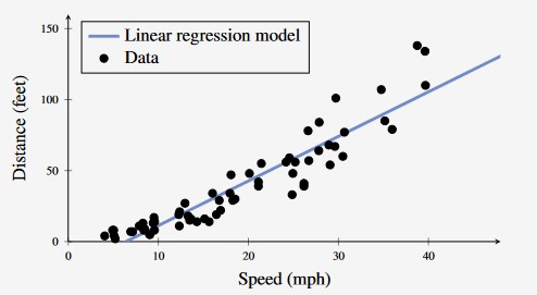
  Figure 1 - Car Stopping Distance with Linear Regression Model

• Lindholm uses the notation $\hat{\theta}_0$, $\hat{\theta}_1$ to denote the y-intercept and gradient respectively

• Fundamentally, the linear regression model is a line/curve fitting model

  • The goal is to capture the general trend of the data
  • However, highly likely that any real-world data will not fit nicely to a line.

• To denote this non-conformance to the straight line, we introduce a term $\varepsilon$ to represent this uncertainty, which represents the additive noise in the system.

$$y=\theta_0 + \theta_1 x_1 + \theta_2 x_2 + \cdots + \theta_p x_p + \varepsilon \tag{3.2}$$

• This equation can be more compactly represented using vector / matrix notation and linear algebra  

$$\begin{align*} y = \theta_0 + \theta_1 x_1 + \theta_2 x_2 + \cdots + \theta_p x_p + \varepsilon = \begin{bmatrix} \theta_0 & \theta_1 & \cdots & \theta_p \end{bmatrix} + \begin{bmatrix} 1\\x_1\\\vdots\\x_p \end{bmatrix} + \varepsilon = \theta^T {\bf{x}} + \varepsilon \end{align*} \tag{3.3}$$

Training a Linear Regression Model

• In training a linear regression model from a set of training data denoted $\mathcal{T}=\lbrace {\bf{x}_i,y_i}\rbrace_{i=1}^n$ we first collect the training data, which is comprised of:

$$X=\begin{bmatrix}{\bf{x}}_1^T\\{\bf{x}}_2^T\\\vdots\\{\bf{x}_n^T}\end{bmatrix}, Y=\begin{bmatrix}y_1\\y_2\\\vdots\\y_3\end{bmatrix}$$

• Note that in the formula, each ${\bf{x}}_i$ is a vector ${\bf{x}}_i=\begin{bmatrix}1 x_{i1}&x_{i2}&\cdots&x_{ip}\end{bmatrix}^T$ of a series of input data points

• The output in this case is a single (numerical) value

• Given this training set, we want to determine the parameters $\theta=\begin{bmatrix}\theta_0&\theta_1\end{bmatrix}^T$ that best fit the data.

• We can use this vector and matrix notation to describe the linear regression model for all training points $x_i, \text{for } i=1,\cdots,n$ in one equation

$$y=\theta^T {\bf{x}} + \varepsilon\tag{3.7}$$

Optimisation of Linear Regression

• A typical machine model has a set of parameters, with which it will predict certain values
• We can find the difference between the predicted value and the true value (ground truth)
• We want to minimise this difference between the predicted value and the truth, and this can be done by changing the model’s parameters.
  • This “difference” is defined by a loss function, denoted $\mathcal{\hat{y}, y}$ which measure how close the model’s prediction $\hat{y}$ is to the observed data / truth $y$.
  • If the model fits well to the data, $\hat{y}\approx y$ then the loss function should have a small value.
• The training of the model can be mathematically defined as:

$$\hat{\theta}=\arg \min_\theta \underbrace{\frac{1}{n} \sum_{i=1}^{n} (\overbrace{\mathcal{L} {\hat{y}({\bf{x}}_i;{\bf{\theta}}), y_i}}^{\text{loss function}} )}_{\text{cost function J(0)}}$$

Least-Squares and the Normal Equations

• A commonly used loss function for regression is the squared error loss, denoted as

$$L(\hat{y}(\bf{x}; {\bf{\theta}}), y)=(\hat{y}({\bf{x};{\bf{\theta}}})-y)^2 \tag{3.10}$$

• This loss function is 0 if $\hat{y}({\bf{x}};\theta)=y$ and grows quadratically as the difference between $y$ and the prediction $\hat{y}$ increases.
  • That is, the loss function is 0 if the prediction matches the ground truth.
• Using the squared error loss, the cost function for the linear regression model given in (Eq 3.7) is given as:

$$\begin{aligned}J(\theta)&=\frac{1}{n}\sum_{i=1}^{n} (\hat{y}(\bf{x}_i;\theta)-y_i)^2\\&=\frac{1}{n} ||{\bf{\hat{y}}}-{\bf{y}}||_2^2 \\&= \frac{1}{n} ||{\bf{X}}\theta-{\bf{y}}||_2^2 \\&=\frac{1}{n}||\bf{\epsilon}||_2^2\tag{3.11}\end{aligned}$$

• This squared error loss can be visualised below, where the squared error loss is the sum of area of squares.

  • Observe that points which are further away from the line have significantly larger squares.
  • This means that the squared error loss function is potentially sensitive to outliers.

  

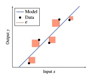
  Figure 2 - Squared Error Loss Visualisation.

• In the end, when we are trying to train a ML model, we are trying to find the optimal $\hat{\theta}$ that minimises the error.

• This can be denoted as follows:

$$\hat{\theta}=\arg\min_\theta=\frac{1}{n}\sum_{i=1}^{n}(\theta^T{\bf{x}}_i-y_i)^2=\arg\min_\theta\frac{1}{n}||{\bf{X}}\theta-{\bf{y}}||_2^2\tag{3.12}$$

• If ${\bf{X}}^T{\bf{X}}$ is invertible, then there exists a closed-form equation (we can solve it in a single step, using linear algebra) instead of using some sort of iterative search algorithm
• The algorithm for solving this is given as

$$\hat{\bf{\theta}} = ({\bf{X}}^T{\bf{X}})^{-1} {\bf{X}}^T y \tag{3.14}$$

Maximum Likelihood Perspective

Turns out to be equivalent to the Sum of Squared Error perspective.

• The Maximum Likelihood framework is used to fit models to data in statistics

  • Important to incorporate statistics in to Machine Learning as we use statistics to handle the uncertainty in the data.
  • Use the terminology “Maximum likelihood” to refer to finding the value of $\theta$ that makes observing $\bf{y}$ as likely as possible.

• If we assume that our model parameters are instances of random variables, then the likelihood function is something that is sensible to optimise (maximise) to build a good model for the data

• If we assume that the noise term $\varepsilon$ is normally distributed, then minimising the squared error loss is equivalent to maximising the log likelihood

• To do this, we want to find some $\hat{\bf{\theta}}$ using the following formula:

$$\hat{\theta} = \arg \max_\theta p({\bf{y}} | {\bf{X}} ; \theta)\tag{3.15}$$

• Here $p({\bf{y}} | {\bf{X}}; \theta)$ is the probability density of all observed outputs $\bf{y}$ in the training data, given all inputs $\bf{X}$ and parameters $\theta$.
• As mentioned before, our noise term $\varepsilon$ has a normal / Gaussian distribution with a mean of zero and variance $\sigma_\varepsilon^2$

$$\varepsilon ~ \mathcal{N}(0, \sigma_\varepsilon^2) \tag{3.16}$$

• Assuming that all $n$ observed training points are independent, and so, $p({\bf{y}}|\bf{X};\theta)$ factorises as:

$$p({\bf{y}} | {\bf{X}};\theta)=\prod_{i=1}^n p(y_1 | {\bf{x}}_i, \theta)\tag{3.17}$$

• Combining the linear regression model equation (Eq 3.3) with the Gaussian noise assumption (Eq 3.16) gives our probability distribution equation:

$$\begin{align*} p(y_i | {\bf{x}}_i, \theta)&=\mathcal{N}(y_i;\theta^T {\bf{x}}_i, \sigma_\varepsilon^2)\\ &=\frac{1}{\sqrt{2\pi\sigma_\varepsilon^2}} \exp({-\frac{1}{2\sigma_\varepsilon^2} (\theta^T {\bf{x}_i} - y_i)^2}) \end{align*}\tag{3.18}$$

• If our noise is randomly distributed, it is a bit of a simplification that our model predicts a single value (our best-guess / average value of where the prediction should be).
  • We should instead predict the confidence interval for these values to model this normally distributed uncertainty.
  • (Eq. 3.18) gives the probability distribution for the prediction.
• Decreasing the error is equivalent to taking the derivative of the equation and solving for when the error is 0.
  • In this case, we are solving for $\hat\theta$.
• In this case, the optimisation of the equation below is equivalent to optimising the equation without the logarithm
  • This is useful, as the multiplication of small number results in increasingly small numbers (may result in increasingly small numbers)
  • To get around this, take the logarithm of the function
  • This only works as a logarithm is a monotonically increasing function

$$\ln p ({\bf{y}} | {\bf{X}} ; \theta) = \sum_{i=1}^n \ln p (y_i | {\bf{x}}_i, \theta) \tag{3.19}$$

• We can remove the factors and terms independent of $\theta$ (which do not change the maximising argument) to derive the following equation

$$\begin{align*} \hat{\theta} &=\arg\max_\theta p({\bf y}|{\bf{X}};\theta)\\ &=\arg\max_\theta -\sum_{i=1}^n(\theta^T {\bf{x}}_i-y_i)^2\\ &=\arg\min_\theta\frac{1}{n} \sum_{i=1}^n (\theta^T {\bf{x}}_i - y_i)^2\tag{3.21} \end{align*}$$

Observe that this is exactly the sum of squared error term we obtained earlier.

Linear Classification / Logistic Regression

How do we deal with categorical input variables using the linear regression model

• Logistic Regression is just linear regression, in which the output variable is categorical, $[0,1]$.
• Therefore, we need to add a squashing function (e.g. sigmoid) to constrain the output to lie in this range.

Key Points

• Logistic regression fits nicely within the Maximum Likelihood framework

• Training the model requires an iterative/numerical optimisation algorithm (unlike linear regression, which has a closed-form solution as a result of introducing the non-linearity).

• We can use one-hot encoding and a logistic regression model.

• For example, for a classification problem with two classes $\lbrace\text{A, B}\rbrace$ we denote the encoding as the creation of a dummy variable which we can use for supervised machine learning

$$x= \begin{cases} 0&\text{if A},\\ 1&\text{if B} \end{cases} \tag{3.22}$$

• If a categorical variable takes more thant two values, say, $\lbrace\text{A, B, C, D}\rbrace$, we can make the one-hot encoding by constructing a four-dimensional vector in which only one of the values are 1 and the rest are 0
  • For example, if the class is $\text{A}$ then $x_A=1$ and the rest are 0.

$${\bf{x}} = \begin{bmatrix} x_A & x_B & x_C & x_D \end{bmatrix}^T \tag{3.24}$$

Binary Classification Problem

• In a binary classification with two input variables $\begin{bmatrix} x_1 & x_2 \end{bmatrix}$, the decision boundary is visualised as below

  

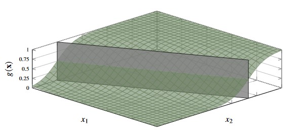
  Figure 3 - Decision Boundary of 2-class problem with two input variables.

• If $g({\bf{x}})>0.5$ then predict class $1$, else predict class $-1$ (or class $0$ depending on labelling scheme)

  • We could also determine the probability that a given input belongs to a certain class (this is why we discuss linear regression and classification through the lens of Maximum Likelihood)
  • It is in fact more powerful to have a classifier that returns the probability and a prediction, rather than just the prediction itself.
    • It tells you how confident the model is in its prediction

Squashing Linear Regression

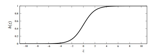
Figure 4 - Logistic Function

• We can use the logistic function to “squash” the output from the linear regression model to be in the range $[0,1]$

Classification Notation

• For binary classification problems ($M=2$) where $y\in\{-1, 1\}$ we train a model $g({\bf{x}})$ for which:

p(y=1 | {\bf{x}}) \text{ is modelled by } g({\bf{x}}) \tag{3.26a}

• We can use $p(y=1|{\bf{x}})$ to compute $p(y=-1|{\bf{x}})$ as by the laws of probabilities $p(y=1|{\bf{x}})+p(y=-1|{\bf{x}})=1$

p(y=-1|{\bf{x}})\text{ is modelled by } 1-g({\bf{x}}) \tag{3.26b}

• For a multi-class problem, we let the classifier return a vector-valued function, where:

$$\begin{bmatrix} p(y=1|{\bf{x}})\\ p(y=2|{\bf{x}})\\ \vdots\\ p(y=M|{\bf{x}})\\ \end{bmatrix} \text{ is modelled by } \begin{bmatrix} g_1({\bf{x}})\\ g_2({\bf{x}})\\ \vdots\\ g_M({\bf{x}}) \end{bmatrix} =\bf{g(x)}\tag{3.27}$$

Model Notation

• We begin constructing the logistic regression / classification model by starting with the linear regression model

$$z = \theta_0 + \theta_1 x_1 + \theta_2 x_2 + \cdots + \theta_p x_p =\theta^T \bf{x}\tag{3.28}$$

• We can then “squash” the output of this model using the logistic function
  • Note that in this function we can omit the noise term as the randomness in classification is statistically modelled by the class probability construction $p(y=m|{\bf{x}})$ instead of an additive noise variable $\varepsilon$.

$$g({\bf{x}}) = \frac{e^{z}}{1 + e^{z}}\tag{3.29a'}$$

* A modified version of Eq 3.29a from Lindholm et al

Training the Logistic Regression Model

In short, we can train the logistic regression model using the principle of maximum likelihood.

The only difference is that the model is denoted slightly differently.

• The training of the model is effectively solving Eq 3.30 shown below

$$\hat{\theta}=\arg\max_\theta p({\bf{y}} | {\bf{X}} ; \theta) = \arg\max_\theta \sum_{i=1}^n \ln p(y_i | {\bf{x}}_i; \theta)\tag{3.30}$$

• In which the log likelihood component can be denoted as:

$$\begin{align*} J(\theta) &=-\frac{1}{n}\sum\ln p(y_i|{\bf{x}}_i;\theta)\\ &=\frac{1}{n}\sum_{i=1}{n} \underbrace{ \begin{cases} -\ln g({\bf{x}}_i;\theta)&\text{if }y_i=1\\ -\ln (1-g({\bf{x}}_i;\theta))&\text{if }y_i=-1\\ \end{cases}}_{\text{Binary cross-entropy loss }\mathcal{L}(g({\bf{x}_i;\theta}),y_i)} \end{align*}\tag{3.32}$$

• Note here that the loss that we have derived is the binary cross-entropy loss.
  • This is a good loss function to optimise given that it corresponds directly to the maximum likelihood principle

Multi-Class Logistic Regression

• Instead of having a scalar-valued function $g({\bf{x}})$ representing $p(y=1|{\bf{x}})$ we have a vector-valued function ${\bf{g}}({\bf{x}})$ which represent the individual class probabilities.
  • The Softmax function here is a normalised version of the logistic function shown above.
• Each of the entries in the vector is an instance of the logistic regression function, each denoted $z_m$, each with their own set of parameters $\theta_m, z_m=\theta^T_m{\bf{x}}$.
• We stack all instances of $z_m$ into a vector of logits ${\bf{z}}=\begin{bmatrix}z_1&z_2&\cdots&z_M\end{bmatrix}^T$ and use the soft-max function to replace the logistic function

$$\text{softmax}({\bf{z}})\overset{\Delta}{=} \frac{1}{\sum_{m=1}^{M} e^{z_m}} \begin{bmatrix} e^{z_1} & e^{z_2} & \cdots e^{z_M} \end{bmatrix}^T \tag{3.41}$$

• We now have a combined expression for linear regression and the softmax function to model the class probabilities

$${\bf{g}}({\bf{x}})=\text{softmax}({\bf{z}}), \ \ \ \ \ \ \ \ \ \ \ \ \ \text{where }\bf{z}= \begin{bmatrix} \theta_1^T{\bf{x}}\\ \theta_2^T{\bf{x}}\\ \vdots\\ \theta_M^T{\bf{x}}\\ \end{bmatrix} \tag{3.42}$$

• We can equivalently write out the class probabilities (elements of vector ${\bf{g}}({\bf{x}})$) as:

$$g_m({\bf{x}})=\frac{e^{\theta^T_m {\bf{x}}}}{\sum_{j=1}{M} e^{\theta^T_j {\bf{x}}}}, \ \ \ \ \ \ \ \ \ \ \ \ \ \ \ \ \forall m=1, \cdots, M \tag{3.43}$$

• We use the multi-class cross-entropy loss function shown below

$$J(\theta)=\frac{1}{n}\sum_{i=i}^{n} \underbrace{-\ln g_{y_i} ({\bf{x}}_i;\theta)}_{\text{Multi-class cross-entropy loss}}\tag{3.44}$$

• Note that this multi-class cross-entropy loss is denoted $\mathcal{L}({\bf{g}}({\bf{x}}_i;\theta),y_i)$
• We can insert the model we developed in (Eq 3.43) into the loss function (Eq 3.44) to give the cost function to optimise for the multi-class logistic regression problem.

$$J(\theta)=\frac{1}{n}\sum_{i=1}^{n}(-\theta_{y_i}^T {\bf{x}}_i + \ln \sum_{j=1}^{M} e^{\theta_j^T{\bf{x}}_i})\tag{3.45}$$

• We optimise this cost function iteratively to train the logistic regression model.’

  

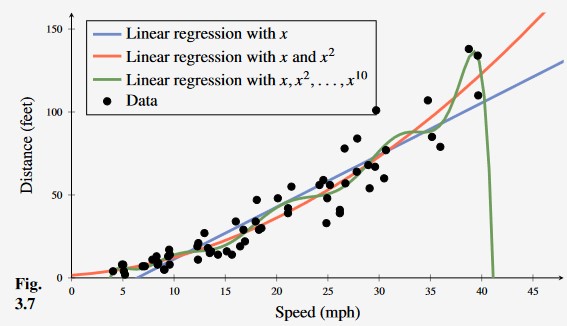
  Figure 4 - Learning the car stopping distance with linear regression, second-order polynomial regression and 10th order polynomial regression. From this, we can see that the 10th degree polynomial is over fitting to outliers in the data making it less useful than even ordinary linear regression (blue).

• On the training set, we can prove that the 10th order polynomial has the lowest error / is the most accurate on the training set.

  • However, this is not necessarily a good thing - the 10th order polynomial is over fitting to the data.