COMP4702 Lecture 4

Error Function

• An error function $E(\hat{y}, y)$ compares the predicted value $\hat{y}$ with the true value $y$ in which a smaller value is better.

  • We have already seen a few error functions, such as Sum of Squared Error (SSE) and Misclassification Rate.

• The error function can be the same as the loss function, but isn’t necessarily the same.

  • Loss function used for training the model
  • Error function used to evaluate a trained model

• The ultimate goal in Machine Learning is to build models that predicts the results of new, unseen data well

  • We assume that this data follows some unknown distribution $p({\bf{x}},y)$ that is stationary
  • We also assume that data points are drawn randomly from this distribution

• Our goal is to minimise the expected new error data $E_\text{new}$ which is the expectation of all possible test data points with respect to its distribution &nbsp

$$E_{\text{new}} \overset{\Delta}{=} \mathbb{E}_\star [ E ( {\color{lightblue}\hat{y}({\bf{x_\star}}; \mathbb{T}), y_\star})]\tag{4.2}$$

• This is expressed as &nbsp

$$\mathbb{E}_\star [ E ( {\color{lightblue}\hat{y}({\bf{x_\star}}; \mathbb{T}), y_\star})]=\int E({\color{lightblue}\hat{y}({\bf{x_\star}};\mathcal{T}), y_\star}) p({\bf{x_\star}},y_\star) d{\bf{x_\star}} dy_\star \tag{4.3}$$

• Here we use the integral symbol to denote that we perform many repeated evaluations.

• Recall here that $\color{lightblue}\hat{y}$ is our model.

• In addition to the introduction of $E_\text{new}$ we introduce the training error $E_\text{train}$: &nbsp

$$E_\text{train} \overset{\Delta}{=} = \frac{1}{n}\sum_{i=1}^n E(\hat{y}({\bf{x}}_i;\mathcal{T}), y_i)\tag{4.4}$$

Motivation for Estimating E_new

• By estimating E_new, we learn a few key things
• Firstly, it gives us an indication of how well our model will perform in the real world with new, unseen data
  • If the model isn’t “good enough” we can try collecting mode data or changing the model
  • On the other hand, we can use it to tell whether there is a fundamental limitation on the model (e.g., are the classes fundamentally overlapping and we can’t distinguish them)
• We can also use $E_\text{new}$ to compare different models and perform hyperparameter tuning.
  • However, its use in tuning the performance of a model or selecting a model invalidates its use as an estimator of $E_\text{new}$
  • To resolve this, need a new hold-out partition to perform this validation on
• Finally, we can use $E_\text{new}$ to report the expected performance to the end user.

Why E_train isn’t E_new

• Consider the case where we use a form of look-up table as a supervised machine learning model.
• We can store the training data in a table, which would yield $E_\text{train}=0$
• This doesn’t help us predict new data.
• In practice, we often see $E_\text{train} < E_\text{test}$

Estimation via Validation Set

• We can set aside some data points (randomly) and use these to estimate $E_\text{new}$ in what is called the hold-out (or validation) dataset.

  

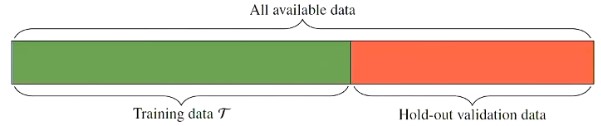
  Figure 1 - Partition of dataset into training and hold-out set.

• Using the hold-out data we can compute $E_\text{hold-out}$ which is an unbiased estimate of $E_\text{new}$

  • As the size of the hold-out validation set increases, $E_\text{hold-out}$ will be a better, lower-variance estimate of $E_\text{new}$
  • However, this leaves less data for training itself.

• There is no “standard” percentage split but most people use 70/30 or 80/20

Estimation via k-Fold Cross Validation

• Randomly partition data into $k$ equally sized subsets

• Then we train the model $k$ times and compute $E_\text{hold-out}$ for each run

  • In the first run, the validation set is the first batch, and the training set is every other batch
  • In the second run, the validation set is the second batch, and the training set is every other batch

  

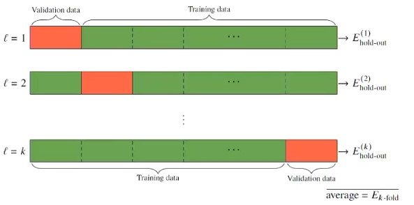
  Figure 2 - k-fold cross-validation

Training Error - Generalisation Gap Decomposition of E_New

• We often see statements about Machine Learning techniques in terms of “it doesn’t work” or “performance is better than human”
• These statements are usually too vague to have much meaning
• To really understand the performance of a Machine Learning model, it is useful to think about the generalisation gap
  • The generalisation gap is a function of our estimates of $\bar E_\text{new}$ and $\bar{E}_\text{train}$

$$\overline{E}_\text{new}\overset{\Delta}{=}\mathbb{E}_{\mathcal{T}}[E_\text{new}(\mathcal{T})]\tag{4.8a}$$

$$\overline{E}_\text{train}\overset{\Delta}{=} \mathbb{E}_{\mathcal{T}}[E_\text{train}(\mathcal{T})]\tag{4.8b}$$

$$\text{generalisation gap}\overset{\Delta}{=}\overline{E}_\text{new}-\overline{E}_\text{train}\tag{4.10}$$

<!-- cSpell: disable-next-line-->
![](/images/notes/COMP4702/overfitting-vs-underfitting.jpg)



<!-- cSpell: disable-next-line-->
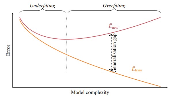
Figure 3 - Behaviour of Enew and Etrain for many supervised machine learning techniques are a function of the model complexity.

• Generally, as the complexity of a model increases, the training error decreases.
• There is a “sweet spot” for $\overline{E}_\text{new}$ in which it is decreased which is denoted by the dotted line in the figure above.
  • It is quite tricky to find this line, but we will discuss ways of approaching it.

Training Error - Generalisation Gap Example

• Consider a binary classification example with a two-dimensional input $\bf{x}=\begin{bmatrix}x_1&x_2\end{bmatrix}$.

• In this simulated example, we know that $p({\bf{x}},y)$ in which $p({\bf{x}})$ is a uniform distribution on the square $[-1,1]^2$ and $p(y|{\bf{x}})$ is defined as follows:

  • All points above the dotted curve in Figure 4 are blue with probability 0.8, and points below the curve are red with probability 0.8

• The optimal classifier, in terms of minimal $E_\text{new}$ would have the dotted line as its boundary and achieve $E_\text{new}=0.8$

  

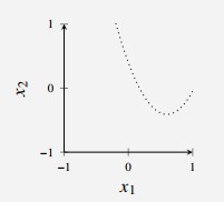
  Figure 4 - Optimal decision boundary for classification problem.

• We then generate this dataset with $n=200$ samples and learn three $k$-NN classifiers with $k=70$, $k=20$ and $k=2$ and plot the decision boundaries.

  

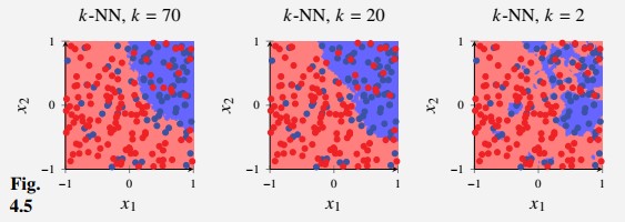
  Figure 4 - Optimal decision boundary for classification problem.

• In this figure, we see that the model $k=2$ adapts too much to the trends in the data

• $k=70$ is rigid enough to not adapt to the noise, but might be a bit too inflexible to adapt to the true dotted line

• We can compute $E_\text{train}$ by counting the fraction of misclassified points.

  • $E_\text{train}=\lbrace 0.27, 0.24, 0.22 \rbrace$

• Since this is a simulated example, we also have access to $E_\text{new}$ which is $E_\text{new}=\lbrace 0.26, 0.23, 0.33 \rbrace$

  • This pattern resembles Figure 3 above, except that $E_\text{new}$ is actually smaller than $E_\text{train}$ for some values of $k$ (this doesn’t contradict the theory).
  • The theory is in terms of $\overline{E}_\text{new}$ and $\overline{E}_\text{train}$ not for $E_\text{train}$ and $E_\text{new}$
  • That is, we need to repeat this experiment ~100 times and compute the average over those experiments.

• This example is positive and increases with model complexity, whereas $\overline{E}_\text{train}$ decreases with model complexity.
• For these values, $\overline{E}_\text{new}$ has a minimum for $k=20$ which suggests that $k=2$ suffers from over fitting and $k=70$ suffers from under fitting

Minimising Training Gap

• We also need to be aware that the size of the dataset affects the size of the generalisation gap

  • Typically, more training data usually means a smaller training data, although $\overline{E}_\text{train}$ probably increases.

• The textbook also discusses minimising $\overline{E}_\text{train}$ whilst having a small generalisation gap and end up with this advice

  • If $E_\text{hold-out}\approx E_\text{train}$ consider that you could be under-fitting. To try improve results, increasing model flexibility.

  • If $E_\text{train}$ is close to zero but $E_\text{hold-out}$ is not, you could be over fitting. To try to improve results, decrease model flexibility

    

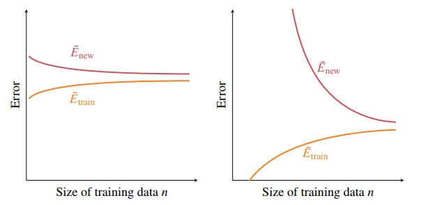
    Figure 5 - Optimal decision boundary for classification problem.

• Simple Model Generalisation gap isn’t so wide but slightly decreases as the size of the training gap decreases.

  • More data to train model $\rightarrow$ model that performs better on the test data.

• Complex Model Same shapes but very different magnitudes

• Intuition $\rightarrow$ small dataset for small models, larger dataset has enough information to train a more complex model.

Example: Training Error vs Generalisation Gap

• Consider a simulated problem so that we can compute $E_\text{new}$.

• Let $n=10$ data points be generated as $x~\mathcal{U}[-5,10]$, $y=\min(0.1x^2,3)+\varepsilon$, $\varepsilon~\mathcal{N}(0,1)$ and consider the following regression methods:

  • Linear Regression with $L^2$ regularisation
  • Linear Regression with a quadratic polynomial and $L^2$ regularisation
  • Linear Regression with a third order polynomial and $L^2$ regularisation
  • Regression tree
  • Random forest with 10 Regression Trees

• For each of these methods, try a few different hyper-parameters (regularisation parameter, tree depth) and compute $\overline{E}_\text{train}$ and the generalisation gap.

  

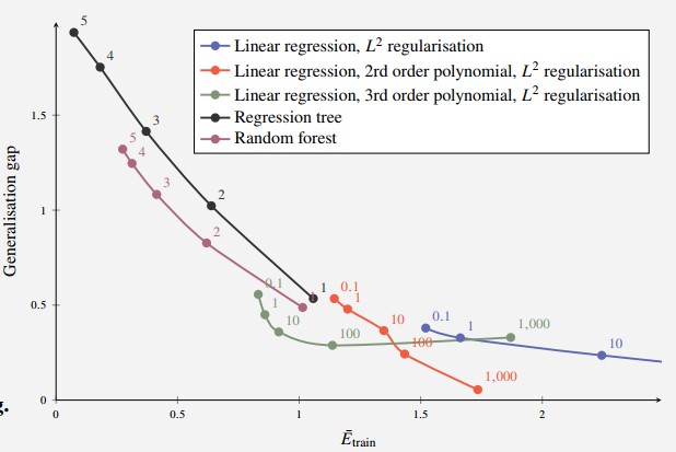
  Figure 6 - Generalisation Gap of Various Models

• Ideally, want both $E_\text{train}$ and the generalisation gap to both be small.

  • In this example, motivated to choose something with small generalisation gap (e.g. 2nd order polynomial linear regression with parameter = 1,000)

• However, note that we can’t plot this against model complexity, as this is very hard to measure in practice

Bias Variance Decomposition of E_new

• Now decompose $\overline{E}_\text{new}$ into statistical bias and variance of the estimates of $E_\text{new}$.
• Suppose we are trying to use a GPS to measure our location.
  • $z_0$ denotes our true location
  • $z$ is the measurement from the GPS which has some random distribution
  • If we read from the GPS several times, we make observations of $z$.
• The mean is given as $\overline{z}=\mathbb{E}[z]$
• Then, we define
  • Bias: $\overline{z}-z_0$
  • Variance: $\mathbb{E}[(z-\overline{z})^2] = \mathbb{E}[z^2]-\overline{z}^2$
• The variance describes the variability in the measurements (e.g., from noise in GPS measurements)
• The bias is some systematic error (e.g. GPS measurements are always offset to one side by a certain amount)

If we knew $z_0$ in reality all of this would be redundant. However, in practice we do not know $z_0$ and therefore we must predict it

• If a model has hyper parameters, it is likely that the complexity of the model can be changed by varying the values of the hyper parameters

  • However, the relationship is often not that simple.

  

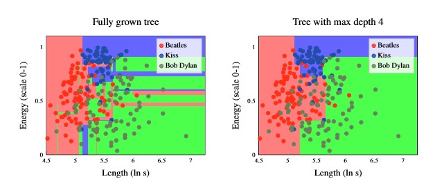
  Figure 7 - Decision boundaries for Decision Trees with different depths

• From the figure above, it is evident that decision trees partition the input space into axis-aligned rectangles.

• Additionally, it is evident that the fully grown tree has a higher model complexity than the tree with max depth of 4.

• The variance depends on the model, but also strongly dependent on the data (the number of data points).

• If we let $n$ denote the size of the training set, it is a bit misleading as the size of the training data is comprised of both rows and columns.

  

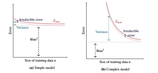
  Figure 8 - Relationship between Bias, Variance and the size of the training set, n

• As the amount of training data increases, the bias and variance decrease

  • We can typically make the model more accurate by collecting more training data
  • Complex models with small amounts of training data can be dangerous, as we have such a large variance component.

  

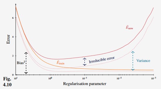
  Figure 9 - Effect of regularisation on error in polynomial regression model.

• Regularisation tends to make models simpler, and thus decrease variance and increase bias.

  

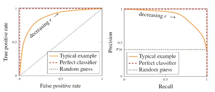
  Figure 10 - ROC (left) and Precision-Recall curves are two types of curves used to evaluate the performance of different classifier cut-offs.

Example 4.5

• UCI Machine Learning Repository for thyroid problems

• 7,200 data points with 21 medical inputs (features) and three diagnoses classes $\lbrace\text{normal, hyperthyroid, hypothyroid}\rbrace$.

• To convert this to a binary classification problem, transform this to the classes $\lbrace\text{normal, abnormal}\rbrace$

• The problem is imbalanced since only 7% of the data points are abnormal

  • Therefore, the naive classifier which always predicts points are normal would obtain a ~7% misclassification rate

• The problem is possibly asymmetric

  • False Positives (falsely predicting the disease) is better than Falsely claiming that the patient is normal
  • Can run diagnoses to more accurately determine that the patient is healthy

• Using the dataset with a logistic regression classifier ($r=0.5$) gives the following result

• Most validation data points are correctly predicted as normal
  • Much of the abnormal data is also falsely predicted as normal (237)
• Lowering the decision threshold $r=0.15$ gives the following confusion matrix

• This gives more true positives (85 v 13) but this happens at the cost of more false positives (111 vs 1)
  • The accuracy is lower (0.919 vs 0.927) but false positives decreased (237 vs 165)