COMP4702 Lecture 5

• Focused on the learning problem in machine learning which is almost always driven by optimisation

Principles of Parametric Modelling

• General expression for regression model $y=f_\theta({\bf{x}})+\varepsilon$.
  • Attempting to model the relationship between inputs and outputs with a function that has parameters $\theta$.
  • Assume additive noise $\varepsilon$.
• In the case of Linear Regression, we know:
  • The model output is a linear function of the parameters
  • The model can be trained in one step, with a closed-form solution using the least-squares error function
  • Assuming Gaussian noise, minimising SSE is equivalent to using the maximum likelihood principle
• However, we want to train non-linear models, using various loss functions (and perhaps different noise assumptions)
• Non-linear models are often used, where the model parameters have a particular meaning - however in ML this is usually not the case.
• Conceptually can replace the linear function in linear regression, and the logit in logistic regression with some other non-linear function $f_\theta({\bf{x}})$ and things still fit in the maximum likelihood framework
• To learn the model, we then need to solve an optimisation problem (Eq 5.4) as a proxy for what we really want to optimise (Eq 5.5)
• Not just a simple matter of solving a numerical optimisation problem
  • Optimisation on training set beyond a certain point isn’t going to help - training set is finite sample
  • The evaluation function (error) might be different from the loss function used for training
    • Some ability to control model complexity (e.g., through explicit regularisation, such as $L_2$ )
  • Early stopping is one way to achieve good generalisation, by not allowing the optimisation to progress all the way to a solution

$$\hat\theta=\arg\min_\theta\underbrace{\frac{1}{n}\sum_{i=1}^{n}\mathcal{L}\overbrace{(y_i,f_\theta({\bf}_i))}^{\text{loss function}}}_{\text{cost function } J(\theta)}\tag{5.4}$$

• Equation 5.4 is the optimisation function in machine learning
  • The optimisation problem is quite tricky to solve, as the optimal solution isn’t exactly what we want
  • We really want to minimise the error on new, unseen data

Loss Functions and Likelihood-Based models

• Different loss functions used in machine learning

• Different properties, useful in different situation

• Given specific information, some combinations of model + loss function make more sense than others

• For regression, we have seen squared error $L_2$ which corresponds to maximum likelihood with Gaussian Noise assumption as shown in Equation 5.6

  $$\mathcal{L}(y,\hat{y})=(\hat{y}-y)^2\tag{5.6}$$

  • Absolute error $L_1$ is more robust to outliers (as it grows more slowly for large errors) and can help with model complexity

  $$\mathcal{L}(y,\hat{y})=|\hat{y}-y|\tag{5.7}$$

  • However, may require different optimisation techniques
  • Additionally consider Huber loss and $\epsilon$-insensitive loss

  

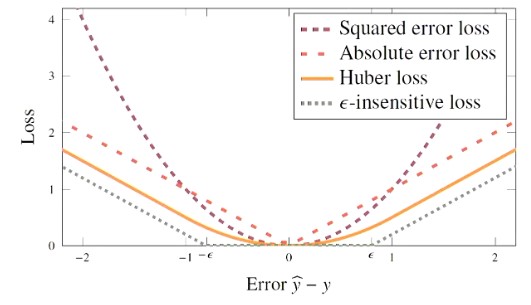
  Figure 1 - Loss Functions for regression presented, as a function of error

• For classification, misclassification loss is intuitive but not often directly used

  • One reason os that this results in a cost function that is piecewise constant - not friendly to numerical optimisation that use gradient info.
  • For a binary classifier that predicts conditional probabilities $p(y=1|{\bf{x}})$ in terms of a function $g({\bf{x}})$ then optimise cross-entropy loss (through maximum likelihood framework)

• Can also work with a measure of how close the (training) data points are to the decision boundary (aka margin)

• If we can bring that information into the loss function, we can train a model to maximise the margin (e.g. SVMs)

• If we think about logistic regression, then we end up making a (hard) class prediction by threshold-ing the logit $\theta^T\bf{x}$ to convert into class predictions -1 and +1.

$$\hat{y}(\bf{x})=\text{sign}\lbrace f({\bf{x}}) \rbrace = \text{sign} \lbrace {{\bf{\theta}}^T{\bf{x}}}\rbrace$$

• The margin of a classifier for a data point $({\bf{x}},y)$ is $y \cdot f({\bf{x}})$
• There are several loss functions that include the concept of margin.
  • Some allow for a probabilistic interpretation of the prediction, some don’t

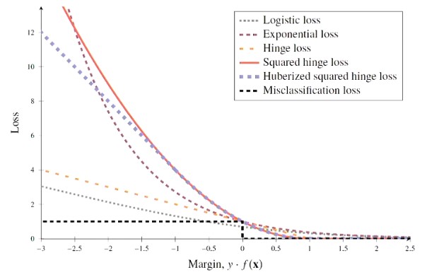
Figure 2 - Loss Functions for Classification

• For multi-class classification, cross-entropy is straightforward, but loss functions that use margin are not.
• In practice, two ways to tackle these problems:
  • One-vs-rest-train: Train $M$ binary classifiers, each one predicting one of the classes vs all the others
    • To predict a point, evaluate each classifier and use the prediction with the greatest margin
  • One-vs-one: Train a classifier to discriminate between every pair of classes (with $\frac{1}{2}M(M-1)$ pairs)
    • To predict a point, evaluate each classifier and take a majority vote. Use margin to break tie.

Note: We leave the next two sections of the book as optional reading

Regularisation

• Regularisation: Some strategy for controlling modelling complexity.
  • Penalise models that are getting too complex.
• Regularisation can be either implicit or explicit

Explicit Regularisation

• Adding a penalty term to the cost function.
• $L^2$ regularisation adds penalty term to the cost function that is the squared $L^2$-norm of the model parameters, with a hyperparameter $\lambda\ge0$ to weight the influence of this term.
  • In Linear Regression, this is called Ridge Regression
  • In Neural Networks, this is called weight decay
• We add the term $\color{lightblue}\lambda || \theta ||_2^2$ on to the end of the regularisation problem

$$\hat\theta=\arg\min_\theta\frac{1}{n} || {\bf X\theta-y}||_2^2 + \lambda || \theta ||_2^2\tag{5.22}$$

• $L^1$ regularisation adds the $L^1$-norm (usually called the Manhattan distance / Lasso).
  • This is more complex to optimise, but has the advantage that it tends to favour sparse solutions where some of the models become (exactly) zero.
  • This is like feature selection for free!

$$\hat\theta=\arg\min_\theta\frac{1}{n} || {\bf X\theta-y}||_2^2 + \lambda || \theta ||_1\tag{5.25}$$

Implicit Regularisation

• Implicit regularisation doesn’t add an explicit term to the cost function, but tries to control model complexity some other way.
• We will see a few examples of explicit regularisation in this course:
  • Early stopping: If training means running an iterative optimisation, monitor $E_\text{hold-out}$ and stop training when it achieves a minimum value
  • Dropout (for Neural Networks)
  • Data augmentation
  • Splitting criterion in decision trees? (Model hyperparameter can also have a regularisation effect.)

Parameter Optimisation

• Certain types of optimisation are heavily used in machine learning

• Most important of optimisation techniques are numerical optimisation techniques, that use gradient information to try and find a good solution

• There are other techniques not mentioned in the textbook, including derivative free methods, metaheuristics (e.g., evolutionary algorithms), linear programming, integer programming.

• The textbook highlights two types of optimisation problems:

  1. Training a model
  2. Hyperparameter optimisation (tuning)

Examples of Objective Functions

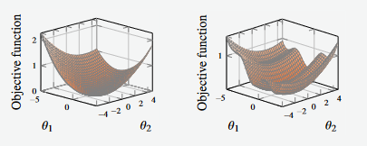
Figure 3 - Example of Objective Functions plotted in 3d

• The goal of training our model is attempting to find the $\theta$ values that allow the objective function to be minimised.

• The function shown on the left is a convex function, and it has a unique global minimum (simple function to optimise)

• The function shown on the right has three local minima, one of which is the global minimum (more complex function to optimise)

• We need an optimisation function or algorithm that can (iteratively) search the surfaces defined by the functions, seeking out the global minimum

  • Note that these functions cannot see the entire surface as we are able to see here - realistically, they are only able to see one point at a time.

• The contour plots of the functions shown above are given below.

  

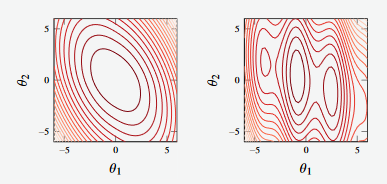
  Figure 4 - Contour plots of functions shown in Figure 3

• Convex functions are easier to optimise from a machine learning perspective

  • Some convex functions have closed-form solutions (e.g., linear regression) but not all do (e.g. logistic regression)
  • In the case where we don’t have a closed-form solution, we require an iterative algorithm to solve it.

Gradient Descent

• One of the oldest optimisation techniques.
• Used in cases where we have functions that we can calculate the gradient of.
• Gradient descent iterates by taking a step in the direction of the negative gradient.

(A note on the optimisation of parameters from first principles)

• For linear regression with squared error loss, training the model amounts to solving the following equation (given that ${\bf{X}}^T\bf{X}$) is invertible

$$\hat\theta=\arg\min_\theta\frac{1}{n} ||{\bf{X}} \theta-{\bf{y}}||_2^2 \tag{3.12}$$

• We can efficiently implement the optimisation algorithm for some of the loss functions in the case of linear regression.
• However, this is not always the case, and for a lot of cases, iterative solutions must be found.
• The generalised parameter learning algorithm is given as

$$\hat\theta=\arg\min_\theta J(\theta) \tag{5.28}$$

• We can use gradient descent to (iteratively) learn parameter vectors $\theta$ when the objective function $J(\theta)$ is simple enough such that its gradient is possible to compute.
• Assume that the gradient of the cost function $\nabla_\theta J(\theta)$ exists for all $\theta$.
• For example, the gradient of the cost function for logistic regression (Eq 3.34) is given as

$$\nabla_\theta J(\theta)=-\frac{1}{n}\sum_{i=1}^{n} (\frac{1}{1 + e^{y_i \theta^T {\bf{x}_i}}}) y_i {\bf{x}}_i\tag{5.29}$$

• Note that $\nabla_\theta J(\theta)$ is a vector of the same dimension as $\theta$ that describes the direction in which $J(\theta)$ increases.

Gradient Descent Algorithm

• The gradient descent algorithm is given as:
• Input: Objective function $J(\theta)$, initial $\theta^{(0)}$ and learning rate $\gamma$
• Result: $\hat{\theta}$

1. Set $t\leftarrow 0$
2. While $||\theta^{(t)} - \theta^{(t-1)}||$ not small enough, do
3.     Update $\theta^{(t+1)}\leftarrow\theta^{(t)}-\gamma\nabla_\theta J(\theta^{(t)})$
4.     Update $t\leftarrow t+1$
5. end
6. return $\hat\theta\leftarrow\theta^{(t-1)}$

• Note To use the gradient descent technique we need an objective function and an initial guess for our parameters

• The key to this algorithm is step (3).

  • We update the new parameter vector using the old parameter vector, moving in the direction of the negative gradient $-\nabla_\theta J(\theta^{(t)})$ by a distance proportional to $\gamma$.

  

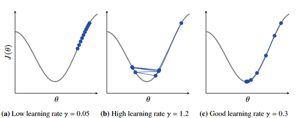
  Figure 5 - Effect of learning rate on finding global minima

• In the figure shown above, we can see the effect of different learning rates.

  • In (a) We see that the learning rate is too low, and approaches the minima too slowly
  • In (b) We see that the learning rate is too high and the function does not reach the minima efficiently.
  • In © We see a good learning rate for the problem

• The size of the learning rate $\gamma$ is very much dependent on the shape of the cost function.

  • In this example $\gamma=0.3$ is a good value, but this may be too small (or too large) for another cost function.

• Observe that in (b) that as the gradient increases, the step size increases.

  • The distance moved is the product of the learning rate $\gamma$ and the local gradient

• Likewise in © as you approach the minima, the gradient decreases and the step size decreases

• Within Line (3) of the algorithm sometimes people perform an internal optimisation problem solved at each iteration to find the optimal $\gamma$.

  • This is a so-called line-search problem

Gradient Descent Example

Example 5.5

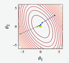
Figure 6 - Convex function

• In the example above, we see two attempts (green and blue lines) to reach some global minima.

• Both attempts reach the global minimum

  

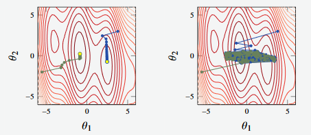
  Figure 7 - Non-Convex function

• However, in Figure 7, we see attempts to find the global minimum on two non-convex functions

• The optimiser doesn’t always find the global minima (in the case of the blue line)

• Furthermore, in the image to the right, the learning rate is too large, and the algorithm doesn’t converge (where we observe strange oscillatory behaviour).

Other Methods

• Second-order gradient methods (e.g. Newton’s method) use second derivative (curvature) information to try to improve the optimisation performance
  • Add considerable complexity and don’t always produce good results.
• Example 5.7 shows us how early stopping can work, and reminds that we don’t actually want the best solution (global optimum) of our training problem.

Early Stopping with Logistic Regression

An example of regularisation by early stopping

• Consider the music classification problem (Example 2.1)
• Apply multi-class logistic regression with a 20-degree polynomial input transformation which gives a model denoted

$$\theta_0 + \theta_1 x_1 + \theta_2 x_2 + \theta_3 x_1^2 + \theta_4 x_1x_2 + \theta_5 x_2^2 + \cdots + \theta_{299} x_1 x_2^{19} + \theta_{230} x_2^{230}$$

• This model has 231 parameters, and with a limited amount of training data, this will likely lead to over-fitting if no regularisation is used.

  

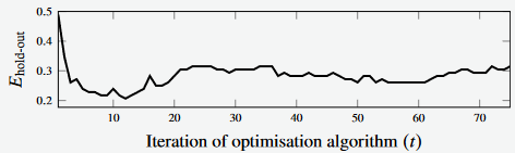
  Figure 8 - Hold-out error

• Figure 8 shows the hold out error for the multi-class classification problem

• Whilst it doesn’t show the loss of the model per iteration, we would expect the loss function to decrease over time.

• The hold-out error goes down but then back-up

  • The minimum hold-out error occurs at Iteration 12, which suggests that after that point, over-fitting occurs and we should probably hav estopped training at that point.

Optimisation with Large Datasets

• When training ML models, objective function usually contains a term that is the sum over all data-points in the training set.
• Important idea - being able to approximate using a subsample of the data-points
• One approximation for this is stochastic gradient descent
  • Can get a good enough approximation of the gradient from a subsample (mini-batch) of the dataset
  • Greater computational efficiency
  • Controversial argument that the noise is able to help the algorithm escape bad solutions during training.
• if each loop of gradient descent updates on a mini-batch the once we have worked through the entire dataset, it is called an epoch.
• The equations for stochastic gradient descent are given as shown in the equations below, where each mini-batch is half of the dataset.

$$\theta^{(t+1)}=\theta^{(t)} - \gamma \frac{1}{n/2} \sum_{i=1}^{\frac{n}{2}} \nabla_\theta\mathcal{L}({\bf{x}}_i, {\bf{y}}_i, \theta^{(t)})\tag{5.37a}$$

$$\theta^{(t+2)}=\theta^{(t+1)} - \gamma \frac{1}{n/2} \sum_{i=\frac{n}{2}+1}^{n} \nabla_\theta\mathcal{L}({\bf{x}}_i, {\bf{y}}_i, \theta^{(t+1)})\tag{5.37b}$$

• The algorithm for stochastic gradient descent is largely the same as gradient descent, but introduces an additional loop to deal with the mini-batches

  • Iterations are renamed to epochs

• In Neural Networks and deep learning, there have been many variations of Stochastic Gradient descent algorithms for training.

  • Many of these algorithms include different techniques for adjusting the step size (learning rate) during training

• The ADAM optimiser is the most widely-used optimiser in deep learning

  • It combines gradient and learning rate values from previous

Hyperparameter Optimisation

• As we employ more ML techniques, we end up with more hyper-parameters that we need to find the optimal value of

• The hyper-parameters of a ML model are typically a collection of different terms that are probably a mix of discrete and continuous values.

• Trying all combinations of several different values for each parameter (grid search) is common but expensive if we have a ot of hyper-parameters (Example 5.9 and Algorithm 5.4).

• This is where black-box or meta-heuristic optimisation algorithms have been successfully applied (e.g., AutoML)