COMP4702 Lecture 8

Bagging and Boosting

• Create a predictor by building a collection (or committee) of base models and combining them together
• Produces favourable properties that mean they often achieve excellent performance

Bagging

Borrowing the idea of bootstrapping from statistics

• Recall the bias-variance tradeoff - complex models potentially good for solving challenging problems and have low bias but have the potential to over fit to training data.
• Bagging (bootstrap aggregating) is a resampling technique that reduces the variance of a model without increasing the bias.

Bootstrapping

• A more general idea from computational statistics to quantify uncertainties in statistical estimators

• Given a dataset $\mathcal{T}$, create multiple datasets $\mathcal{T}^{(1)},\cdots,\mathcal{T}^{(B)}$ by sampling with replacement from $\mathcal{T}$.

• Bootstrapped dataset will have multiple copies of some data points and miss some others but many statistical properties preserved.

• Assume that the size of every bootstrapped dataset is equal to the size of the original dataset

• The bootstrapping algorithm is as follows:

Data: Training dataset $\mathcal{T}=\lbrace{\bf{x}}_i,y_i\rbrace_{i=1}^{n}$

Result: Bootstrapped data $\tilde{\mathcal{T}}=\lbrace\tilde{\bf{x}}_i, \tilde{y}_i\rbrace_{i=1}^{n}$

1. For $i=1,\cdots, n$ do
2.  |   Sample $\ell$ uniformly on the set of integers $\lbrace1,\cdots,n\rbrace$
3.  |   Set $\tilde{\bf{x}}_i={\bf{x}}_\ell$ and $\tilde{y}_i=y_\ell$
4. end

• Essentially, create a “bootstrapped” dataset by sampling with replacement from the original dataset $\mathcal{T}$

Bootstrapping Example

• Consider a dataset generated from some (unknown) function denoted by the dotted line in the figure below.

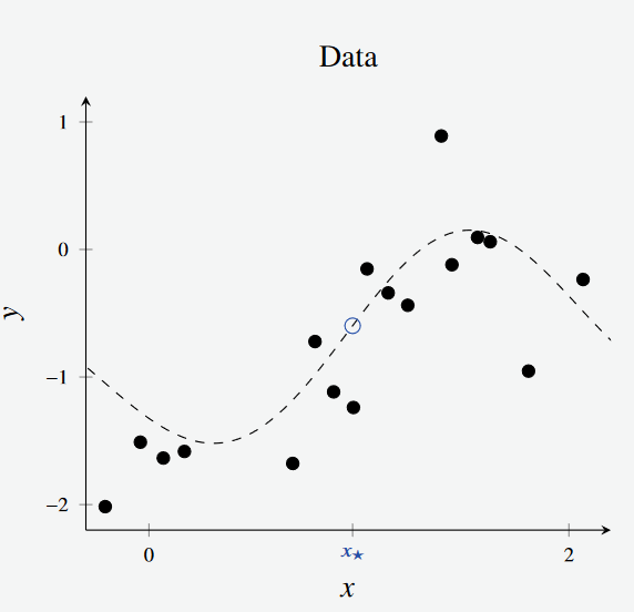
Figure 1 Visualisation of Data for Bootstrapping Example 

• From this dataset, we sample with replacement and create nine bootstrapped regression trees

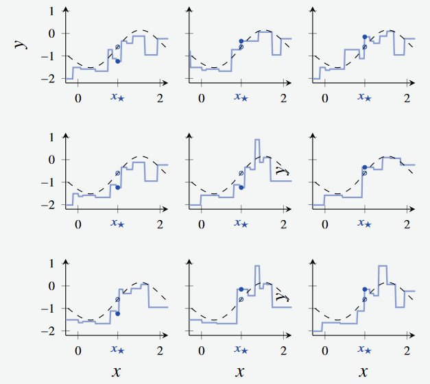
Figure 2 Created 9 bootstrapped trees from the above dataset 

• We can see that the bootstrapped model fits the curve much better.
  • Furthermore, in the regression tree learned from all the data, the prediction point $x_\star$ is quite far away from its true value.
  • The error is decreased when predicting using the bootstrapped regression trees.

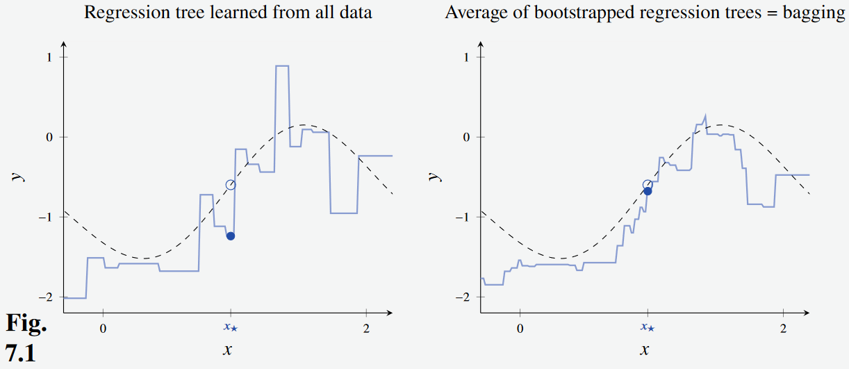
Figure 3 Observe that the resulting model (Right) 

• The technique of bagging creates $B$ bootstrapped datasets, and trains $B$ base models - one on each dataset.

• For each prediction, the predictions of the base models are combined together to form an ensemble.

• For regression or class probabilities, the output is the average of the base models’ prediction

  $$\hat{y}_\text{bag}({\bf{x}_\star})=\frac{1}{B}\sum_{b=1}{B} \tilde{y}^{(b)}({\bf{x}_\star}) \ \ \ \ \ \ \ \ \ \text{or} \ \ \ \ \ \ \ \ \ {\bf{g}}_\text{bag}({\bf{x}_\star})=\frac{1}{B}\sum_{b=1}{B}\tilde{{\bf{g}}}^{(b)}({\bf{x}_\star}) \tag{7.1}$$

• For hard classification labels, take a majority vote of all base models.

How does Bagging reduce the variance of models?

• Consider a collection of random variables $z_1,\cdots,z_B$.
  • Let the mean and variance of these variables be $\mu$ and $\sigma^2$
  • Let average correlation between pairs be $\rho$
• Mean and the variance of these variables (e.g., ensemble output) given by Equation 7.2a and 7.2b

$$\mathbb{E}=\left[\frac{1}{B}\sum_{b=1}^{B} z_b\right]=\mu\tag{7.2a}$$

$$\text{Var}=\left[\frac{1}{B} \sum{b=1}{B} z_b\right]=\frac{1-\rho}{B} \sigma^2 + \rho\sigma^2\tag{7.2b}$$

• We can see that:

  • The mean is unaffected
  • The variance decreases as $B$ increases
  • The less correlated the variables are, the smaller the variance

• Typically, the test error of the ensemble will decrease as the size of the ensemble increases

  • We can see this in Example 7.3, where an increase in the size of the ensemble decreases the squared test error.

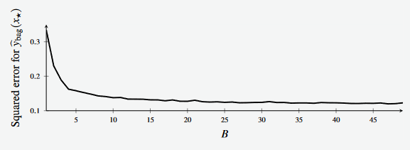
Figure 3 Observe that the resulting model (Right) 

• In practice, this is slightly more difficult:
  • We can’t directly control the correlation between base models, but we might try to encourage them to be somehow less correlated.
    • The randomness from re-sampling will produce some differences between the base models.
  • There could still be overfitting from the base models.
  • Compared to using the original dataset, the bias of the base models might increase because of the bootstrapping

Out-of-Bag Error Estimation

• Bagging is another technique that spends more computational effort to get improvements in models (or estimation)
  • Recall cross-validation as a way to get an estimate of $E_\text{new}$.
• If we produce an ensemble via bagging, each base model will have seen (on average) about 63% of the datapoints.
  • We can use the other $\approx\frac{1}{3}$ of the points to build up an estimate of $E_\text{new}$ called the out-of-bag error $E_\text{OOB}$.
• Each datapoint gets used as a test point for $\approx\frac{B}{3}$ base models, and we average those estimates over all of the datapoints.
• The training computation was already done, so no extra effort is needed compared to cross-validation
• Interestingly, cross-validation is typically used more than $E_\text{OOB}$

Random Forests

• Random forests are bagged decision trees, but with extra trick to try and make base model less correlated.
• At each step when considering splitting a node, we only consider a random subset of $q<p$ variables to split on.
• This might increase the variance of each base model, but if the decrease in $\rho$ is larger then we still get a benefit.
• In practice, people often find that this is the case.
• While $q$ is a hyperparameter (that needs to be tuned), rules of thumb are to use $\lfloor q \rfloor = \sqrt p$ for classification and $\lfloor q \rfloor = \frac{p}{3}$ for regression.

Random Forest v Bagging Example

Example 7.4 from Lindholm et al.

• We have a synthetically generated dataset with points and a decision boundary (denoted by the dotted line)

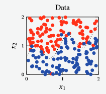
Figure 4 - Dataset for random forest vs bagging example. 

Boosting

• Another ensemble technique, focused on combining simple (likely high bias) base models to reduce the bias of the ensemble.
• The training of models in bagging is parallel.
• Boosting constructs an ensemble sequentially - each model is encouraged to try and focus on mistakes made by previous model(s).
  • Done by weighting datapoints during re-sampling and prediction.
  • This means that it cannot be done in parallel

Example: Bagging vs Boosting

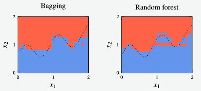
Figure 5 - Decision boundary for a random forest and bagged decision tree classifier 

• The individual ensemble members are given as:

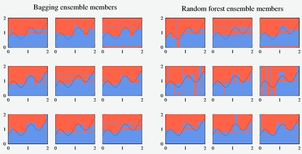
Figure 6 - Compilation of ensemble members for bagging and random forest 

• And likewise, the error rate of the two models

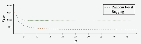
Figure 7 - E new for the random forest and bagging models. 

• Surprisingly, the new error is lower for the random forest than the random forest.
• As $B\rightarrow\infty$ both models’ error decrease.
• However, the Random Forest model’s error continues to decrease after $B=3$ whereas the bagging model seems to stagnate.

Example: Boosting Minimal Example

• Consider a classification problem with two-dimensional input space ${\bf{x}}=\begin{bmatrix}x_1&x_2\end{bmatrix}$
• The training data consists of $n=10$ datapoints (5 samples from each class)
• For example, use a decision stump (decision tree with depth 1) as a simple, weak classifier.

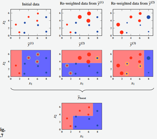
Figure 8 - E new for the random forest and bagging models. 

• In the first iteration of the decision stump, the model misclassifies three of the red points.
• In the second iteration, two red points misclassified
• In the third iteration, three blue points misclassified.
• Use these learnings in creating the final boost model.

Adaboost

An old boosting algorithm that is still quite useful.

• Try to be a little more active about creating an ensemble that creates a better base model when compiled together
• Looking at the pseudocode we can see that
  • Each datapoint is given a weight parameter $w_i$, set initially to be equal
  • Another parameter $a^{(b)}$ is calculated on each iteration using training error.
    • This parameter is then used to modify the weight values to be used in the next iteration
    • The weights are also re-normalised
    • The $a^{(b)}$

The AdaBoost training algorithm is given as:

Data: Training data $\mathcal{T}-\lbrace{\bf{x}}_i, y_i\rbrace_{i=1}^{n}$

Result: $B$ weak classifiers

1. Assign weights $w_i^{(1)}=\frac{1}{n}$ to all datapoints
2. for $b=1,\cdots,B$ do
3.  |    Train a weak classifier $\hat{y}^{(b)}({\bf{x}})$ on the weighted training data denoted $\lbrace ({\bf{x}}_i, y_i, w_i^{(b)})\rbrace_{i=1}^{n}$
4.  |    Compute $E_\text{train}^{(b)}=\sum_{i=1}^{n} w_i^{(b)} \mathbb{I}\lbrace y_i\ne\hat{y}^{(b)}({\bf{x}}_i)\rbrace$
5.  |    Compute $\alpha^{(b)}=0.5\ln((1-E_\text{train}^{(b)})/E_\text{train}^{(b)})$
6.  |    Compute $w_i^{(b+1)}=w_i^{(b)} \exp (-\alpha^{(b)} y_i \hat{y}^{(b)}({\bf{x}})), y=1,\cdots,n$
7.  |    Set $w_i^{(b+1)}\leftarrow =w_i^{(b)} / \sum_{j=1}^{n}$ (normalisation of weights)

From lines 5 and 6 of the AdaBoost algorithm, we cna draw the following conclusions:

• Adaboost trains the ensemble by minimising an exponential loss function of the boosted classifier at each iteration - the loss function is shown in Equation 7.5 below.

  $$L(y \cdot f({\bf x})) = \exp (-y \cdot f({\bf x})) \tag{7.5}$$

  • The fact that this is an exponential function makes the math work out nicely.
• Part of the derivation shows that we can do the optimisation using the weighted misclassification loss at each iteration (Line 4).

Design Choices for Adaboost

• The book gives a few bits of advice for choosing the base classifier and the number of iterations $B$ for AdaBoost:
  • A good idea to use a simple model that’s fast to train (e.g. decision stumps or a small decision tree) because boosting reduces bias efficiently. Note that boosting is still an Ensemble method that uses sampling, so it still possibly reduces variance.
  • Overfitting is possible if $B$ gets too large - could use early stopping.

Gradient Boosting

A newer technique compared to AdaBoost

• AdaBoost uses an exponential loss function that can be sensitive to outliers, noise in the data.
• One way to address this is to use a different loss function (but requires re-thinking of the model)
• If we take a general view of a model (aka function approximator) as a weighted sum combining together some other functions, we have an additive model (statistics term)

$$f^{(B)}({\bf x}) = \sum_{b=1}^{B} \alpha^{(b)} f^{(b)}({\bf x})\tag{7.14}$$

In boosting:

• Each base model/basis function is itself a machine learning model, which has bene learned from data.
• The overall model is learnt sequentially, over (B) iterations

Training via Gradient Boosting

• Training an additive model is an optimisation problem over $\lbrace a^{(b)}, f^{(b)}({\bf x})\rbrace_{b=1}^{B}$ to minimise Equation 7.15 shown below.

$$J(f({\bf X}))=\frac 1n \sum_{i=1}^{n} L(y_i, f({\bf x}_i)) \tag{7.15}$$

• This is done greedily at each step for the exponential loss function in AdaBoost (Equation 7.5)
• Alternatively, any method that will improve $J()$ will be fine (Equation 7.16, 7.17)
  • The base model at step $(b)$ is related to the base model at step $(b-1)$, in which $\alpha$ acts like a step size parameter

    $$f^{(b)}({\bf x}) = f^{(b-1)}{\bf x} + \alpha^{(b)} f^{(b)}({\bf x}) \tag{7.16}$$

  • Then, if our goal is to reduce the objective function, we require that the new value of the objective function to be smaller than that of the previous ensemble to be.

    $$J\left(f^{(b-1)}({\bf X}) + \alpha^{(b)}f^{(b)}({\bf X})\right) < J \left( f^{(b-1)} ({\bf X})\right)$$

• A general approach for this is summarised as:

  • The gradient of, $J()$ with respect to the current base models $(b-1)$ is taken as the gradient of the los function for the base models on the data as shown in Equation 7.18

  • (That is, this method doesn’t necessarily have to be greedy)

  • If we can determine what the gradient of $J()$ is, we can “go downhill” on that gradient to minimise its value.

    $$\nabla _c J(c^{(b-1)}({\bf X})) \overset{\text{def}}{=} \begin{bmatrix} \frac{\partial J(f({\bf x}))}{\partial f({\bf x}_1)} \\ \vdots \\ \frac{\partial J(f({\bf x}))}{\partial f({\bf x}_n)} \\ \end{bmatrix} _ {| \ f({\bf X}) = f^{(b-1)} ({\bf X})} = \frac 1n \begin{bmatrix} \frac{\partial L(y_1, f)}{\partial f} _ {f = f^{(b-1)} ({\bf x}_1)} \\ \vdots \\ \frac{\partial L(y_n, f)}{\partial f} _ {f = f^{(b-1)} ({\bf x}_n)} \\ \end{bmatrix} \tag{7.18}$$

  • Practical implementations of gradient boosting (using decision trees as base models) are often found to give State of the Art performance, with implementations such as XGBoost and LightGBM