COMP4702 Lecture 10

Chapter 9: Bayesian Approach and Gaussian Process Bayesian Inference

The Bayesian Idea

“The statistical methodology of Bayesian learning is distinguished by its use of probability to express all forms of uncertainty. Learning and other forms of inference can then be performed by what in theory are simple applications of the rules of probability. The results of Bayesian Learning are expressed in terms of a probability distribution over unknown quantities. In general, these probabilities can be interpreted only as expressions on our degree of belief in the various probabilities.” - Radford Neal

• A core problem in ML is to be given some data, we want to build a model of the unknown entity that generated the data.
• Assume our model has parameters $\theta$. We have seen that the maximum likelihood estimation provides a principled way to learn $\theta$ from our data.
  • To this point, we claim with 100% certainty that $\theta$ are the optimal parameters, in a problem with much certainty.
  • Furthermore, we only observe a limited (finite) subset of training data.

$$L(\theta|\mathcal{X})\propto p(\mathcal{X}|\theta)=\prod_{i=1}^{n} p({\bf x}_i|\theta)\tag{1}$$

• In the equation $\mathcal{X}$ denotes the training set.
• If we assume all training points are IID, then we can write the likelihood as a product of individual likelihoods.
• But why should we be absolutely certain about our model parameters?
  • Bayesian learning works with a probability distribution over model parameters that expresses our beliefs regarding ow likely different parameter values are.
• We start by defining a prior distribution $p(\theta)$ expressing our belief about the model parameters before we have seen any data.
• After seeing some data, we update our prior to a posterior distribution using Bayes rule:

$$P(\theta|\mathcal{X})=\frac{p(\mathcal{X}|\theta)p(\theta)}{p(\mathcal{X})}\propto L(\theta|\mathcal{X})p(\theta)\tag{2}$$

That is, $\text{posterior}\propto \text{likelihood} \times \text{prior}$

• This is the proper way to combine our prior knowledge with the information obtained from the data.
  • So then, to make predictions about a new data point $x_\star$, a Bayesian ideally uses the posterior predictive distribution

$$p(x_\star | \mathcal{X}) = \int p(x_\star | \theta) p (\theta | \mathcal{X})\ d\theta\tag{3}$$

• To get the probability, we multiply the likelihood term with the posterior distribution (Equation 2) and evaluate over all possible values of $\theta$
• So, we use all $\theta$ weighted by our model posterior (i.e., we average over our uncertainty in estimating $\theta$)
• You can sometimes solve this (e.g., for Gaussian processes) but it is not always easy to solve.
  • If you are fully Bayesian, you would use a Markov-Chain Monte Carlo (MCMC) method to sample from this.
  • Alternatively, the Maximum A-Posteriori (MAP) estimate is often used, which is the mode of the posterior
  • If the prior is uniform over all $\theta$, then the MAP estimate is equal to the maximum likelihood estimate.

Bayesian Linear Regression

Taking the concept of linear regression from before, and using it with Bayesian Inference.

• First, let’s have a look at how Bayesian inference works for linear regression (where the posterior is simple and easy to calculate.)

Multivariate Gaussian Distribution

• We need multivariate probability distributions, but we can pretty much get by with one type: a multivariate Gaussian (Normal) distribution.
• The univariate Gaussian distribution is defined as follows, with parameters $\mu$ (mean) and $\sigma$ (standard deviation):

$$p(z)=\frac{1}{\sigma\sqrt{2\pi}}\exp{-\frac12\left(\frac{z-\mu}{\sigma}\right)^2}$$

• If $\bf z$ is a $q$-dimensional random vector, then a multivariate Gaussian distribution is parameterised by a $q$-dimensional mean vector $\bf \mu$ and $q\times q$ dimensional covariance matrix $\bf \Sigma$.

$${\bf\mu}= \begin{bmatrix} \mu_1\\\mu_2\\\vdots\\\mu_q \end{bmatrix}, \ \ \ \ \ \ \ \ \ \ \ {\bf\Sigma}= \begin{bmatrix} \sigma_1^2 & \sigma_{12} & \cdots & \sigma_{1q}\\ \sigma_{21} & \sigma_2^2 & & \sigma_{2q}\\ \vdots & & & \vdots\\ \sigma_{q1} & \sigma_{q2} & \cdots & \sigma_q^2 \end{bmatrix}$$

• The covariance matrix is a real-valued, positive semidefinite matrix (a symmetric matrix with non-negative eigenvalues).
• One way to make this Gaussian distribution simpler, is to have the only non-zero entries on the covariance matrix on the diagonal.
  • That is, remove the covariance between the different variables.
• Gaussian distributions have lots of useful mathematical properties and are a good model for real-world (continuous) data in lots of situations.

• Recall that in Chapter 3, that our setup for linear regression included additive Gaussian noise (Equation 9.6).

$$y=f({\bf x}) + \varepsilon, \ \ \ \ \ \ \ f({\bf x})=\theta^T {\bf x}, \ \ \ \ \ \ \ \ \varepsilon \sim \mathcal{N}(0,\sigma^2),\tag{9.6}$$

• So we can write the predictive distribution as a Gaussian for a single point (Equation 9.7).
  • Note this is really substituting $f({\bf x})=\theta^T{\bf x}$ into the Gaussian noise term, with error bars $\sigma^2$.

$$p(y|\theta)=\mathcal{N}(y;\theta^T{\bf x}, \sigma^2),\tag{9.7}$$

• This can alternatively be written for multiple points (Equation 9.8).

$$p({\bf y}|\theta)=\prod_{i=1}^{n} p(y_i|\theta) = \prod_{i=1}^{n} \mathcal{N}(y_i;\theta^T{\bf x}_i,\sigma^2)=\mathcal{N}({\bf y};{\bf X}\theta,\sigma^2{\bf I})\tag{9.8}$$

• The IID assumption means that this multivariate Gaussian has a diagonal covariance matrix (covariances are all zero)

  • This is why we have $\sigma^2{\bf I}$ in place of the covariance matrix.

• We want to use Bayesian inference, so we need to start by specifying a prior for our model parameters $p(\theta)$ (that is, the coefficients of the linear regression model. These can be positive or negative)

  • Let’s choose this to be Gaussian as well (Equation 9.9), where for example ${\bf\Sigma}_0={\bf I} \sigma_0^2$

    $$p(\theta)=\mathcal{N}(\theta;{\bf\mu}_0,{\bf\Sigma}_0) \tag{9.9}$$

• Bayes’ rule can then be used to calculate the posterior distribution for the model parameters (Equation 9.10):

  $$\begin{align*} p({\bf\theta}|{\bf y})&=\mathcal{N}({\bf\theta};{\bf\mu}_n,{\bf\Sigma}_n),\tag{9.10a}\\ {\bf\mu}_n &= {\bf\Sigma}_n \left( \frac{1}{\sigma_0^2} {\bf\mu}_0 + \frac{1}{\sigma_0^2}{\bf X}^T {\bf y} \right)\tag{9.10b}\\ {\bf\Sigma}_n &= \left( \frac{1}{\sigma_0^2}{\bf I} + \frac{1}{\sigma_0^2}{\bf X}^T {\bf X} \tag{9.10c} \right) \end{align*}$$

• We can also derive the posterior predictive for $f({\bf x_\star})$:

  $$\begin{align*} p(f({\bf x_\star} | {\bf y})) &= \mathcal{N}(f({\bf x_\star}); m_\star, s_\star), \tag{9.11a}\\ m_\star&={\bf x}_\star^T {\bf\mu}_n \tag{9.11b}\\ s_\star&={\bf x}_\star^T {\bf\Sigma}_n {\bf x}_\star + \sigma^2 \tag{9.11c} \end{align*}$$

• We have so far only derived the posterior predictive for $f({\bf x_\star})$.

• Since we have $y_\star=f({\bf x}_\star) + \varepsilon$ according to the linear regression model (Equation 9.10), where $\varepsilon$ is assumed to be independent of $f$ with variance $\sigma^2$, we can also compute the posterior predictive for $\bf y_\star$ as shown in Equation 9.11d below.

$$p(y_\star | {\bf y}) = \mathcal{N}(y_\star; m_\star, s_\star + \sigma^2) \tag{9.11d}$$

• Finally, we can include the noise into the prediction:

$$p({\bf y})=\mathcal{N}\left({\bf y} ; {\bf X\mu}_0, \sigma^2 {\bf I} + {\bf X\Sigma}_0{\bf X}^T\right)\tag{9.12}$$

• The additive noise is on the target values of the data, and its standard deviation is $\sigma$ (which has to be chosen).

• The variance of the prior distribution is $\sigma_0$.

  • These (different) hyper-parameters can be tuned by maximising an optimisation problem, the marginal likelihood $p({\bf y}$), Equation 9.12

• One of the nice things about Bayesian Inference is that we get a predictive distribution, that captures precisely the uncertainty of our predictions, given the prior and the model.

Example 9.1 - Bayesian Linear Regression

We consider a simle one-dimensional example, with

$$y= \theta_1 + \theta_2 x + \varepsilon$$

In this first figure, we see the models generated by sampling from the prior.

![](/images/notes/COMP4702/bayesian-linear-regression-1.png)



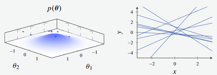
 Figure 1a - Bayesian Linear Regression Prior. (Left): Feature Space, where the features are the intercept and gradient of the line respectively. (Right): Plotted models, with parameters sampled from feature space.

We next see the effect of sampling from the posterior with a single datapoint. Initially, the prior has a broad distribution when no data has been observed.

![](/images/notes/COMP4702/bayesian-linear-regression-2.png)



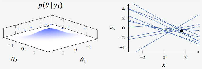
 Figure 1b - Bayesian Linear Regression Posterior with 1 data point. (Left): Feature Space, where the features are the intercept and gradient of the line respectively. (Right): Plotted models, with parameters sampled from feature space.

Extending this, we see the effect when sampling the posterior with three data points, and 30 data points respectively. The distribution continues to shrink as we sample more and more from the data.

![](/images/notes/COMP4702/bayesian-linear-regression-3.png)



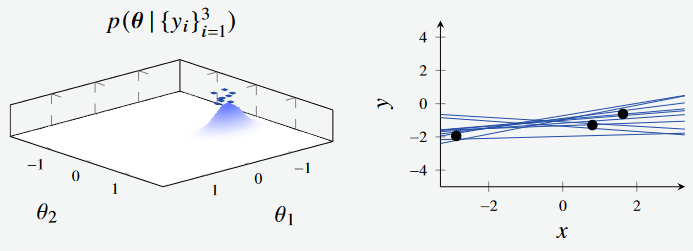
 Figure 1c - Bayesian Linear Regression Posterior with 3 data points. (Left): Feature Space, where the features are the intercept and gradient of the line respectively. (Right): Plotted models, with parameters sampled from feature space.



![](/images/notes/COMP4702/bayesian-linear-regression-4.png)



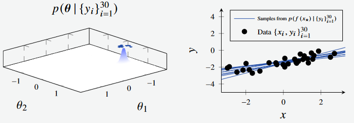
 Figure 1d - Bayesian Linear Regression Posterior with 3 data points. (Left): Feature Space, where the features are the intercept and gradient of the line respectively. (Right): Plotted models, with parameters sampled from feature space.

After sampling 30 data points, the distribution of points are much more concentrated. We can see how the posterior contracts as we sample more data. Also observe how the blue surface becomes more peaked on the left, and the blue lines in the plot to the right becoming more concentrated around the true line.

Example 9.2 - Car Stopping Distances

• Consider the car stopping distance problem, and apply linear regression with a linear and quadratic transformation respectively

$$y=1+\theta_1x + \varepsilon \\ y = 1 + \theta_1 x + \theta_2 x^2 + \varepsilon$$

• We set $\theta^2$ and $\theta_2^2$ by maximising the marginal likelihood, which gives:

  • $\theta^2=12.0^2, \theta_0^2=14.1^2$ for the linear model and

  • $\theta^2=10.1^2, \theta_0^2=0.3^2$ for the quadratic model.

    

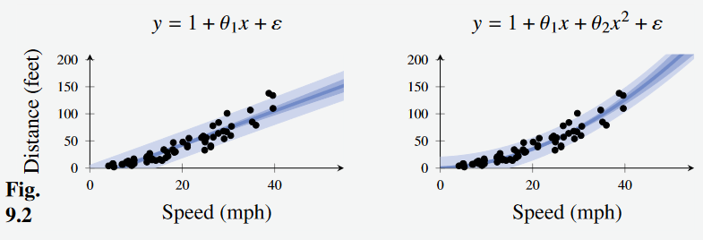
    Figure 2 - Car stopping distance with Bayesian Linear Regression. (Left): Linear transformation. (Right): Quadratic transformation

• The dark blue line in the center shows the mean (i.e. the $y= 1 + \theta_1 x$ component of the linear regression model) and the lighter bars show the standard deviation of the models.

Connection to Regularised Linear Regression

• Previously, we looked at adding $L^2$ regularisation to linear regression.
• When we train by optimising the loss function, we get a point estimate for the model parameters $\hat\theta_{L^2}$.
• For the Bayesian linear regression model we just looked at (Equation 9.9).
• It turns out that $\hat\theta_{L^2} = \hat\theta_{MAP}$ which is the peak of the posterior distribution: the Maximum A-Posteriori solution.
• This is interesting because it shows that the Bayesian approach is doing something like regularisation (making it less prone to overfitting).
• From the other direction, you could say that adding regularisation to a model is like implicitly choosing a prior distribution, but you don’t get the prior distribution unless you “Go Bayesian”.

The Gaussian Process

![](/images/notes/COMP4702/linear-regression-connections.png)



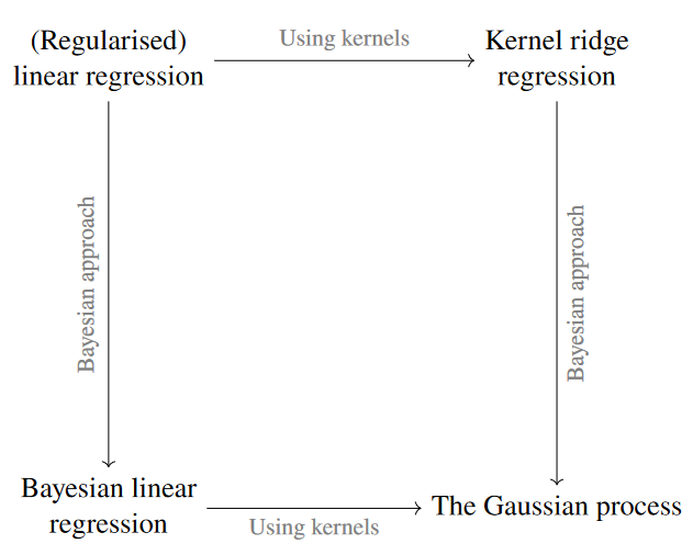
 Figure 3 - Connection of concepts learned so far.

• We began talking about regularised linear regression.
• In the previous lecture, we discussed using Kernel ridge regression, and we just discussed Bayesian linear regression
• In the end, both of these approaches lead us to the Gaussian process.
• The book focuses first on showing why the mathematics underlying Gaussian processes works.
• Let’s simplify and instead focus on the practical aspects of Gaussian processes

• Gaussian Processes (GPs) have a nice Bayesian interpretation.

  • Consider the regression problem - a gaussian Process specifies a prior distribution directly over the function space (instead of model parameters) and does inference with it given some (supervised) training data.
  • Function Space Distribution of possible functions

• To do this, we need to consider more than just random variables; We need to consider stochastic processes

  • Stochastic Process: A collection of random variables $\lbrace Y(x), x\in X\rbrace$ indexed by a set $X$.
  • A stochastic process is specified by giving the joint probability distribution for every finite subset of variables $Y(x_1, \cdots, x_k)$ in a consistent manner.

• For a Gaussian Process, every subset of data points has a multivariate Gaussian distribution

  • To achieve this, we need a mean function and covariance function which fully specify our Gaussian Process.
  • The covariance function $\kappa({\bf x}, {\bf x}')$ represents our prior belief about how we think the value of the function $\bf x$ is affected by the value of the function at $\bf x'$ and vice versa.

• The demo made by the textbook authors here provides an interactive visualisation of the Gaussian Process.

  • Here the squared exponential covariance function is used - one of the most common kernel functions used.
  • Measures the similarity (or dis-similarity) between two datapoints $\bf{x, x}'$.
  • The Kernel function is used here as a means of encoding the prior, influenced by the training points seen.

• That is, if we were to predict some $y$ value at x=10, it likely be more strongly influenced by the close-by observations (e.g., $x=-15, x=0$ in this example) compared to observations that are further away.

  • After specifying the hyper parameters $\sigma, \ell$, we can “train” our Gaussian Process model.

    

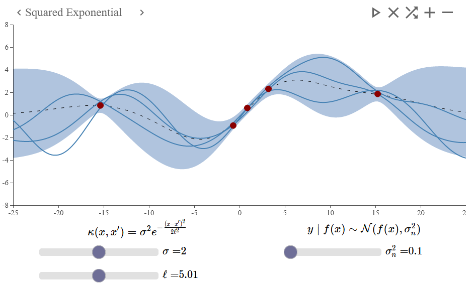
    Figure 4 - Gaussian Process example with a squared exponential covariance function. This was generated using http://smlbook.org/GP/index.html

• One specific benefit of the Gaussian Process is that it encodes the uncertainty, rather than just giving a singular prediction.

  • We are “fairly confident” (that is, we’ve seen data that correlates to this) that the shape in the middle is somewhat sinusoidal.

  • However, we haven’t seen evidence for the behaviour of hte datapoints out toward the edges.

  • This is precisely what is modelled by $s_\star$ of the Gaussian process (blue shaded region) in the figure below

    

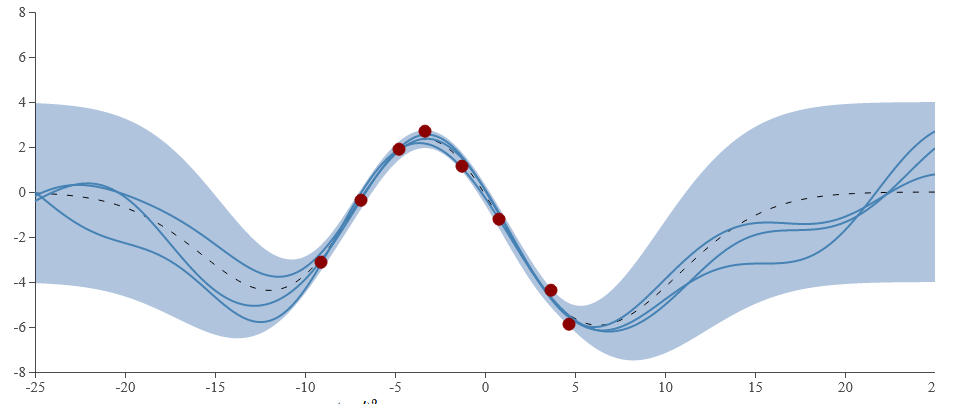
    Figure 5 - Gaussian Process example with a squared exponential covariance function. This was generated using http://smlbook.org/GP/index.html

Training a Gaussian Process Model

• One of the nice things about Gaussian Process models is that they don’t have to be trained - there exists a closed form solution
• We apply the same derivation trick as with kernel ridge regression, replacing all instances of ${\bf\phi}({\bf x})^T{\bf\phi}({\bf x}')$ with a kernel $\kappa({\bf x}, {\bf x}')$.
• With this, we get the following equation, where $m_\star$ denotes the mean (black line in Figure 4), and $s_\star$ denotes the variance (shaded region in Figure 4).

$$m_\star={\bf\Kappa}({\bf X}, {\bf x_\star})^T\left(\sigma^2 {\bf I} + {\bf \kappa} ( {\bf X, X})\right)^{-1}\bf{y}\tag{9.25a}$$

$$s_\star=\kappa({\bf x_\star,x_\star})-{\bf \Kappa}({\bf X, x_\star})^T \left(\sigma^2 {\bf I} + {\bf \Kappa}({\bf X, X})\right)^{-1} {\bf \Kappa}({\bf X, x_\star}) \tag{9.25b}$$

• Note here that $\kappa(x,x')$ is the variance for a single point, and ${\bf\Kappa}({\bf X, X})$ denotes the covariance matrix (where $\bf X$ denotes the training data).

  • This covariance matrix is of dimensionality $q\times q$ where $q$ is the number of training points.
  • In addition to this ${\bf \Kappa}({\bf X, x_\star})$ is a vector of dimensionality $1\times q$, and represents the covariance between the test point, and every training point.
  • Note that in both Equation 9.25a and 9.25b we need to be able to invert matrices - this is hard / ?impossible? if the diagonals are zero, so we add the additive noise term $\sigma^2$ to the diagonal of the covariance matrix.

• $\sigma$ denotes the vertical scale of the uncertainty, and $\ell$ is the “length scale” of the model - how smooth the predictions.data are.

• $\sigma^2$ denotes the uncertainty around the prediction

• Figure 9.3 to 9.5 show how the marginal distribution for one variable is determined by a value observed for another variable.

• The Gaussian Process is a tractable way of extending this idea of slicing up Gaussian distributions (one for each data point) to an infinite number of points using a function

• We end up with a posterior predictive distribution (which of course is Gaussian).

• We start with a prior over the function space.

  • Once some data is observed, we update our prior to get a posterior.

• Our belief about the possible functions have changed - the predictive variance has reduced considerably, especially close to where we observe datapoints.

Drawing Samples from a Gaussian Process

• The posterior predictive distribution for a single point is a univariate Gaussian distribution, but over the whole input space it is a distribution of functions.
• One common way of showing this is to plot a few sample functions from this distribution.
• This isn’t hard to do - take a (test) set of data points, calculate the resulting mean vector and covariance matrix using the kernel.
• Sample $n$ points is equivalent to an $n$-dimensional Gaussian distribution - we then slice this up and plot the values side by side.

Practical Aspects of the Gaussian Process

• To use a Gaussian Process, we have to choose a covariance / kernel function

  • This will have a big impact on the model, resulting prediction and performance.

• Kernel functions will have their own hyper parameters.

• ML Researchers tend to use a couple of general-purpose covariance functions, but there have been lots of variations developed for specific applications and other data settings (e.g., non stationary kernels that are dependent on the specific position in the input space)

• t is possible to optimise the hyper parameters of a covariance function in a principled way by maximizing the (marginal) likelihood (Eqn. 9.27). Figures 9.12 and 9.13 show some examples of this.

  • This is a non-convex optimisation problem but an expression for the gradient is available, so gradient-based methods are typically used. See Example 9.3 for fitting a GP to the car stopping data