COMP4702 Lecture 11

Chapter 10: Generative Models

• Previous chapters have been mostly about supervised learning, which generate models of $p(y|{\bf x})$.
• Generative models are models of $p({\bf x}, y, \theta)$.
  • Dropping the $y$ term would make this unsupervised learning.
• Generative models are very similar to probabilistic models and computer simulation models - they all draw from some probability distribution.
• So we can use a probability density estimation and think of this as a foundation for unsupervised learning and generative models.

Gaussian Mixture Models and Discriminant Analysis

Mixture Densities

• A mixture model is a weighted sum of component densities e.g. this case, Gaussian Distributions

$$p({\bf x})=\sum_{i=1}^{k} p({\bf x}|G_i) P(G_i)$$

• Where $G_i$ is the $i$th component (aka group or cluster assumed to be in the data)
  • $P(G_i)$ is the prior/mixture coefficient or weight of the $i$th component and $p({\bf x} | G_i)$ is the $i$th component PDF.
  • Note that $0 \le P(G_i)\le 1 \forall i$ and $\sum_{i=1}^{k} P(G_i) = 1$.
• We will look at Gaussian Mixture Models (GMMs), so:

$$p({\bf x} | G_i) = \mathcal{N}({\bf \mu}_i, \Sigma_i)$$

• If for a single variable, specify mean and standard deviation.
• If multivariate, specify mean vector and covariance matrix.
• The parameters of our GMM are $\mu_i, \Sigma_i, P(G_i), i=1,\cdots,k$. So the LHS of the above equation is more properly written as:

$$p({\bf x}|\theta)=p({\bf x} | {\bf \mu}, \Sigma_i, P(G_i))$$

![](/images/notes/COMP4702/gaussian-sum.png)


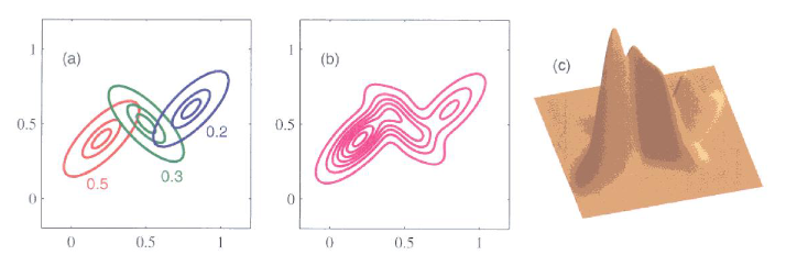
Figure 1 - A Gaussian mixture model with 3 Gaussian distributions in a two-dimensional space.

• The left plot Figure 1 describes that we can write a GMM as the weighted sum of 3 (in this case) Gaussian distributions.
• These three smooth functions add up to create a single smooth function as shown in the center plot of Figure 1.
• This GMM is plotted in three dimensions in the right of Figure 1.

• What happens next is really all about whether or not you know apriori whether your data comes from some groups/categories/classes and if you have those “labels” for your data.

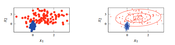
Figure 2 - A Gaussian mixture model with 3 Gaussian distributions in a two-dimensional space.

• The above example assumes that you know the labels $\in \lbrace\text{red, blue}\rbrace$, shown on the left.
• With these knowledge, you can separate these points out and create a Gaussian distribution for each class - shown by the contour lines in the plot to the right.
• The weight of each probability distributed by the frequency of each class in the data.
• Can use Maximum Likelihood Estimation (MLE) to estimate the parameters of each Gaussian distribution.

Predicting Output Labels for New Inputs: Discriminant Analysis

• This section shows that you can use a GMM to do classification, because you can use your model of $p({\bf x},y)$ to get $p(y|{\bf x})$.

  • $\bf x$ being the coordinates and $y$ being the class labels.

• This is a nice illustration for multi-class classification, bu you can just use a single Gaussian distribution for the binary classification and you’d be close to logistic regression

• However, there are a few key differences:

  • Priors: not present in logistic regression. With Logistic Regression, it doesn’t explicitly encode the idea that one class has more samples than the other.

  • Different parametrisations of the covariance matrix give rise to Linear Discriminant Analysis (LDA) or Quadratic Discriminant Analysis (QDA) when you allow covariance modelling.

    • LDA when you have a diagonal Covariance matrix.

    

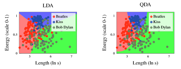
    Figure 3 - Difference in decision boundaries generated by LDAs and QDAs.

• The figure above shows the difference between the decision boundaries generated by Linear Discriminant Analysis (LDA) vs Quadratic Discriminant Analysis (QDA).

  • Observe that in the figure to the left (LDA), the decision boundaries are linear whereas the decision boundaries in the figure to the right (QDA) are quadratic.

Semi-Supervised Learning of the Gaussian Mixture Model.

• Where we have some data that is labelled, but also (probably a lot more) that is unlabelled.
  • We would like to make use of this unlabelled data as well as the labelled data.
• We would like to maximise the likelihood but we can’t do this directly using the unlabelled data as shown in Equation 10.9:

$$\hat\theta=\arg\max_\theta\ln p( \underbrace{\lbrace\lbrace{\bf x}_i, y_i\rbrace_{i=1}^{n_l}, \lbrace{\bf x}_i\rbrace_{i=n_l+1}^{n}\rbrace }_{\tau})| \theta$$

• However, this problem has no closed-form solution
• However, we can take the following approach:
  1. Learn the GMM from he labelled data.
  2. Use the GMM to predict $p(y=m | {\bf x}_i,\hat{\bf\theta})$ as a proxy for the labels for the unlabelled data.
  3. Update the GMM’s parameters including the data with predicted labels.
• This concept works and isn’t just some random idea - it’s a version of the Expectation Maximisation (EM) algorithm
• The equations relevant to this procedure are given as:

$$\begin{align*} w_i(m)&= \begin{cases} p(y=m|{\bf x}_i, \hat\theta) & \text{ if } y_i \text{ is missing}\\ 1 & \text{ if } y_i = m\\ 0 & \text{ otherwise} \end{cases} \tag{10.10a}\\ \hat\pi_m &= \frac{1}{n} \sum_{i=1}{n} w_i(m) \tag{10.10b}\\ \hat\mu_m &= \frac{1}{\sum_{i=1}^{n} w_i (m)} \sum_{i=1}^{n} w_i(m) {\bf x}_i \tag{10.10c}\\ \hat\Sigma_m &= \frac{1}{\sum_{i=1}^{n} w_i (m)} \sum_{i=1}^{n} w_i(m) ({\bf x}_i - \hat\mu_m) ({\bf x}_i - \hat\mu_m)^T \tag{10.10d} \end{align*}$$

Cluster Analysis

• If we do not have a defined target variable (e.g., labels or numerical variables) we are in the realm of unsupervised learning.

• The data consists of observations of features collected from some problem domain, and presumably contains structure and information that is of interest.

• One way to learn about that structure is to build a model of the distribution of the data (i.e. probability density estimation).

• A GMM is a flexible probability density estimator, and peaks of the density give us an understanding of the clustering of data (places in the feature space where data occurs with high probability).

• The EM algorithm can be used to fit a GMM to data for $\bf x$.

  • Effectively $y$ is marginalised out of the estimate $p({\bf x},y)$ and becomes a latent variable for the model.
  • The latent variables are $\lbrace y_i\rbrace_{i=1}^{n}$ where $y_i\in\lbrace 1,\dots,M\rbrace$ is the cluster index for data point ${\bf x}_i$.
  • This algorithm is shown in Method 10.3 below:

Data Unlabelled training data $\mathcal{T}=\lbrace{\bf x}_i\rbrace_{i=1}^{n}$, number of clusters $M$Result Gaussian Mixture Model

1. Initialise $\hat{\bf\theta}=\lbrace\hat\pi_m, \hat{\bf\mu}_m, \hat{\bf\Sigma}_m\rbrace_{m=1}^M$
2. repeat
3.  |   For each ${\bf x}_i$ in $\mathcal{T}=\lbrace{\bf x}_ i\rbrace_ {i=1}^{n}$ compute the prediction $p(y|{\bf x}_ i, \hat{\bf\theta})$ using Equation 10.5 using the current parameter estimate $\hat{\bf\theta}$.
4.  |   Update the parameter estimates $\hat{\bf\theta}\leftarrow\lbrace\hat\pi_m, \hat{\bf\mu}_m, \hat{\bf\Sigma}_m\rbrace_{m=1}^M$ using Equations 10.10.
5. until convergence

• In the “E step” (Line 3) We compute the “responsibility values” - how likely is it that a given data point could have been generated by each of the components of the mixture model? Note that the notation here is quite confusing: $y$ is actually a vector of values for each mixture component.

• In the “M step” (Line 4) we update the model parameters $\bf\theta$ using the responsibility values computed in the E step. Lindholm refer to the responsibility values as weights, $w_i(m)$

• Maximising the likelihood for a GMM is a non-convex optimisation problem, and the EM algorithm performs local optimisation which hopefully converges toward a stationary point

• This works pretty well most of the time, though there is also a degeneracy in the problem - undesirable solutions where the likelihood diverges to infinity.

k-Means Clustering

• We can understand that the $k$-Means clustering algorithm as a simplified version of fitting a GMM using the EM algorithm.
• The simplification made are:
  • Rather than calculating (soft, probabilistic) responsibility values, $k$-Means calculates “hard” responsibility values based on the distances between a point and a set of $k$ cluster centers.
  • The distances in the GMM use the covariance information (i.e. the Mahalanobis distance between each data point and each component of the GMM)
• The algorithm is given as the following steps:
  1. Set the cluster centers $\def\bmu{\bf\mu} \hat\bmu_1, \hat\bmu_2, \cdots, \hat\bmu_M$ to some initial values
  2. Determine which cluster $R_m$ each ${\bf x}_i$ belongs to by finding the cluster center $\hat{\bf\mu}_i$ that is ${\bf x}_i$ for all $i\in\lbrace 1,\dots,n\rbrace$.$
  3. Update the cluster centers $\hat{\bf\mu}_m$ as the average of all ${\bf\mu}_i$ that belongs to $R_m$
  4. Repeat steps 2 and 3 until convergence

Choosing the Number of Clusters

• Unfortunately no simple answer - sometimes problem domain knowledge can guide the choice.