Lecture 1

Nothing important, just admin stuff

Lecture 2

k-Nearest Neighbours

• Prediction determined by looking at labels or true values of $k$ nearest points in training set.
  • Implies some sort of distance metric
• Regression: Use average of $k$ nearest points
• Classification: Use majority vote of $k$ nearest points
• Choice of $k$ should be such that the model neither overfits nor underfits.

Decision Trees

• A model that divides the feature space into axis-aligned regions.
• Learning all possible spaces is intractible, so a greedy algorithm is used
• Regression: Use average of points in region
  • Commonly use Sum of Squared Error as a metric for splitting
• Classification: Use majority vote of points in region
  • Use misclassification rate, Gini index or entropy criterion as a metric for splitting

Lecture 3

Linear Regression

• Training is easy as there eists a closed-form solution
• Use loss function as a metric to measure the similarity between prediction and truth
  • Commonly use Squared Error Loss

Maximum Likelihood Perspective

• Wanting to maximise the probability that our prediction is the observed value (Maximum Likelihood Perspective) turns out to be equivalent to using Squared Error Loss.
• Arrive at the same equation.

Logistic Regression

• Similar to Linear Regression, but with a sigmoid function applied to the output to bound the output between 0 and 1.
• No closed-form solution exists (numerical optimisation required)
• For binary classification, we train a model to predict $p(y=1|{\bf x})$, and then $p(y=-1|{\bf x})=1-p(y=1|{\bf x})$.
• For multi-class problem, we train $K$ linear regression models to predict $p(y=k|{\bf x})$ for $k=1,\ldots,K$ using one-hot encoding.
  • Softmax is used such that the sum of all probabilities is 1.
  • Each output is then the probability that the input belongs to the corresponding class.

Lecture 4

Error Functions

• An error function compares the predicted value $\hat{y}$ with the true value $y$
  • If an error function returns a smaller value, the prediction is better.
  • SSE and Misclassification Rate are examples of Error functions
• Error functions can be the same as the oss function, but isn’t necessarily the same.
  • Loss Function is used for training the model
  • Error function is used to evaluate a trained model

Estimating Enew

• Want to create models that minimise the error over new data
• Use $E_\text{new}$ to compare different models, and perform hyperparameter tuning

1. Estimation via Validation Set
   • Can set aside a portion of the training data as a validation set
   • As the size of the validation set increases, $E_\text{hold-out}$ becomes sa lower-variance estimate of $E_\text{new}$ but this leaves less training data.
2. k-Fold Cross Validation
   • Done by partitioning the dataset into $k$ equally sized subsets, training on $k-1$ subsets and testing on the remaining subset.
   • $E_\text{hold-out}$ is then the average of the $k$ errors.
   • This leads to a lower-variance estimate of $E_\text{new}$ but is more computationally expensive.

Training Error vs Generalisation Gap

• A sweet spot between underfitting and overfitting exists, an equilibrium between model complexity.
• A model with low complexity will have both high E_new and E_train
• A model with high complexity will have high E_new and low E_train
• A model with optimal complexity will have minimal E_new.

Bias-Variance Decomposition of Enew

• $E_\text{new}$ can be decomposed into three components:
  • Bias: The difference between the expected prediction and the true value
  • Variance: The variance of the prediction
• As the amount of training data increases, the bias and variance decrease
  • Typically can make the model more accurate by increasing the amount of training data

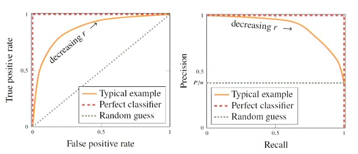
ROC and Precsion-Recall Curves

• Two types of curves that can be used to evaluate the performance of a binary classifier and its different cut-off values

  

Lecture 5

Parametric Modelling

• Want to create and train non-linear models using various loss functions.

Loss Functions

• Regression typically use Squared Error $L_2$, but can also use Absolute Error $L_1$.
  • Absolute error is more robust to outliers and can help with model complexity
• Classification - misclassification loss is intuitive
  • Results in a loss function that is piecewise constant - difficult to optimise as it is piecewise constant
  • Can use cross-entropy loss.

Regularisation

• A strategy for controlling modeling complexity
• Can be either implicit or explicit
• Explicit regularisation works by adding a penalty term to the cost function
  • $L_2$ regularisation is the most common
  • $L_1$ regularisation is also used, but results in a sparse model (where many parameters are 0)
• Implicit regularistaion works by controlling modelling complexity in another way
  • Examples include early stopping, drop-out, data augmentation.

Parameter Optimisation

• The goal of training models is to find $\theta$ that allows the objective function to be minimised
• Gradient descent is one of the oldest optimisation techniques
  • Used where we have functions that we can calculate the gradient of
  • Need to find a learning rate that is suitable - not so low that the model takes a long time to learn, and high that the model cannot approach the minima
• Stochastic gradient descent is a variant of gradient descent that uses a random subset of the training data to calculate the gradient
  • Optimal when optimising a large dataset - the subset is a good enough approximation and leads to greater computational efficiency.

Lecture 6

N/A

Lecture 7

Neural Networks

• Artificial Neuron is a unit that takes in several inputs via weighted connections
  • The output from the neuron is the sum of these weighted inputs (+ bias)
• Each neuron effectively performs linear regression
  • A single layer of units can be trained to perform multiple linear regression (linear regression with multiple outputs)
  • A single layer of units with sigmoid activation function is very similar to multi-class regression
    • (To be identicdal, use Softmax instead of sigmoid)
• Each layer of the neuron network $l$ is parameterised by a weight matrix ${\bf W}^{(l)}$ and a bias vector ${\bf b}^{(l)}$

Training a Neural Network

• Collect all weights and biases and arrange them into a vector $\bf \theta$ to use the same notation as throughout the textbook.
• Use backpropagation to compute the gradient of the MLP via the chain rule
  • To do this, need the partial derivative of $J(\theta)$ with respect to each weight and bias (in each layer of the network).
• Use these partial derivatives to do the update for gradient descent.

CNNs

• Have far fewer parameters than a dense layer, by enforcing structure:
  • Sparse Interactions: The kernel only interacts with a limited local region of inputs
  • Parameter Sharing: The same kernel (learned) is applied to all inputs - less parameters than having a weight for every input.
• Can further reduce the computation is by using stride
  • Move the kernel along by more than 1 unit at a time
• Pooling A layer that has no trainable parameters, but can be used as a component to reduce the size of the model.
  • Done by computing the average (or maximum) values over a given filter size (e.g. $2\times 2$).

Drop-out

• Randomly set some hidden units to 0 each training iteration so that they don’t do anything
• A technique that can reduce model complexity.

Lecture 8

Bagging

• Bootstrapping Create multiple subsets of the data, sampling with replacement from training set.
  • Train a model on each subset of the dataset
  • For each prediction, the base models’ predictions are combined together to form an ensemble.
    • For regression or class probabilities, the output is the average of the base models’ predictions
  • As the size of the ensemble increases, the variance decreases although the mean remains the same
• Random Forest Bagged decision trees, where only a random subset of the nodes are consideed to split on
  • This is in an attempt to make the models less correlated
  • This might increase the variance of each base model, but overall, the random forest should have less variance

Boosting

• A more active approach to ensemble learning
• AdaBoost Iteratively train classifiers, assigning higher weights to points misclassified.
  • The $i$th model uses the weightings provided by the mistakes of the $i-1$th model.
• Want to choose a model that is fast to train
• Can over-fit if $B$ is too large - can use a regularisation technique like early stopping to prevent this.
• Gradient Boosting Use a different loss function that is less sensitive to outliers.
  • Start with a single weak model, and use gradient desent to find the parameters for the next model.

Lecture 9

Kernels

• Define a kernel function $\kappa({\bf x, x'})$ between two datapoints
• Given a set of non-linear basis functions (input transformations), then a very useful kernel function is the inner product between the pairs of datapoints.
• Can use this kernel function to define our model as follows:

$$\def\p{\bf \Phi} \def\X{\bf X} \hat y({\bf x_\star}) = \underbrace{{\bf y}^T}_{1\times n} {\underbrace{\p(\X) \p(\X)^T + n \lambda {\bf I}}_{n\times n}}^{-1} {\underbrace{\p(\X){\bf\phi} ({\bf x_\star})}_{n\times 1}} \tag{8.7}$$

Kernel Ride Regression

• Uses the kernel function across the entire training set $\bf X$ and a test point $\bf x_\star$ denoted $\kappa({\bf X}, {\bf x_\star})$
• Use loss functions that are positive definite kernels such as the Gaussian kernel.
• An advantage of this is that the number of the parameters in the model is relaed to the number of training samples $n$ rather than the number of input features $p$.

Support Vector Regression

• Change the loss function used in Kernel Ridge Regression to $\epsilon$-insensitive loss function
  • This loss function is 0 if the error is less than $\epsilon$ and linearly increasing otherwise.

Kernel Functions

• Can create our own kernel function to describe the similarity between two datapoints.
• In practice, don’t need to worry that the kernels are positive semidefinite (except for kernel ridge regression.)
• Examples of kernels include the linear kernel (Equation 8.23) and the polynomial kernel (Equation 8.24) in which the order of the polynomial is $d-1$

$$\kappa({\bf x, x}')={\bf x}^T{\bf x}'\tag{8.23}$$

$$\kappa({\bf x, x}')=(c +{\bf x}^T{\bf x}')^{d-1}\tag{8.24}$$

Support Vector Classification

• If using the hinge loss function then we end up with a training problem that is convex-constrained optimisation problem
  • Requires numerical solver
  • when this is solved, the solution tends to be sparse, with many $\alpha_i=0$

Lecture 10

Bayesian Approach

• A statistical approach for finding optimal parameter set $\bf\theta$ for the model.

1. Define prior distribution $p({\bf\theta})$ over the parameters before seeing data
2. Observe some data and update the prior to a posterior distribution $p({\bf\theta} | {\bf X})$
3. To make predictions about a new datapoint $\bf x_\star$ multiply the likelihood with the posterior distribution and integrate (evaluate) over all parameters

Bayesian Linear Regression

• Can get away with multivariate gaussian distribution
• There’s a closed-form solution
• Get a predictive distribution that captures the uncertainty given the prior and model
• Sampling more datapoints from the training set causes the predictive distribution to converge to the true solution
  • Uncertainty around the observed points reduces.
• For linear regression, can use linear and quadratic kernels.

Lecture 11